
MATH 233 - Linear Algebra I
Lecture Notes
Cesar O. Aguilar
Department of Mathematics
SUNY Geneseo
Lecture 0
Contents
1 Systems of Linear Equations 1
1.1 What is a system o f linear equations? . . . . . . . . . . . . . . . . . . . . . . 1
1.2 Matrices . . . . . . . . . . . . . . . . . . . . . . . . . . . . . . . . . . . . . . 4
1.3 Solving linear systems . . . . . . . . . . . . . . . . . . . . . . . . . . . . . . 5
1.4 Geometric interpretation of the solution set . . . . . . . . . . . . . . . . . . 8
2 Row Reduction and Echelon Forms 11
2.1 Row echelon form (REF) . . . . . . . . . . . . . . . . . . . . . . . . . . . . . 11
2.2 Reduced row echelon for m (R REF) . . . . . . . . . . . . . . . . . . . . . . . 13
2.3 Existence and uniqueness of solutions . . . . . . . . . . . . . . . . . . . . . . 17
3 Vector Equations 19
3.1 Vectors in R
n
. . . . . . . . . . . . . . . . . . . . . . . . . . . . . . . . . . . 19
3.2 The linear combination problem . . . . . . . . . . . . . . . . . . . . . . . . . 21
3.3 The span of a set of vectors . . . . . . . . . . . . . . . . . . . . . . . . . . . 26
4 The Matrix Equation Ax = b 31
4.1 Matrix-vector multiplication . . . . . . . . . . . . . . . . . . . . . . . . . . . 31
4.2 Matrix-vector multiplication and linear combinations . . . . . . . . . . . . . 33
4.3 The matrix equation problem . . . . . . . . . . . . . . . . . . . . . . . . . . 34
5 Homogeneous and Nonhomogeneous Systems 41
5.1 Homogeneous linear systems . . . . . . . . . . . . . . . . . . . . . . . . . . . 41
5.2 Nonhomogeneous systems . . . . . . . . . . . . . . . . . . . . . . . . . . . . 44
5.3 Summary . . . . . . . . . . . . . . . . . . . . . . . . . . . . . . . . . . . . . 47
6 Linear Independence 49
6.1 Linear independence . . . . . . . . . . . . . . . . . . . . . . . . . . . . . . . 49
6.2 The maximum size of a linearly independent set . . . . . . . . . . . . . . . . 53
7 Introduction to Linear Mappings 57
7.1 Vector mappings . . . . . . . . . . . . . . . . . . . . . . . . . . . . . . . . . 57
7.2 Linear mappings . . . . . . . . . . . . . . . . . . . . . . . . . . . . . . . . . 58
7.3 Matrix mappings . . . . . . . . . . . . . . . . . . . . . . . . . . . . . . . . . 61
7.4 Examples . . . . . . . . . . . . . . . . . . . . . . . . . . . . . . . . . . . . . 62
3

CONTENTS
8 Onto, One-to-One, and Standard Matrix 67
8.1 Onto Mappings . . . . . . . . . . . . . . . . . . . . . . . . . . . . . . . . . . 67
8.2 One-to-One Mappings . . . . . . . . . . . . . . . . . . . . . . . . . . . . . . 69
8.3 Standard Matrix of a Linear Mapping . . . . . . . . . . . . . . . . . . . . . . 71
9 Matrix Algebra 75
9.1 Sums of Matrices . . . . . . . . . . . . . . . . . . . . . . . . . . . . . . . . . 75
9.2 Matrix Multiplication . . . . . . . . . . . . . . . . . . . . . . . . . . . . . . . 76
9.3 Matrix Transpose . . . . . . . . . . . . . . . . . . . . . . . . . . . . . . . . . 80
10 Invertible Matrices 83
10.1 Inverse of a Matrix . . . . . . . . . . . . . . . . . . . . . . . . . . . . . . . . 83
10.2 Computing the Inverse of a Matrix . . . . . . . . . . . . . . . . . . . . . . . 85
10.3 Invertible Linear Mappings . . . . . . . . . . . . . . . . . . . . . . . . . . . . 87
11 Determinants 89
11.1 Determinants of 2 × 2 and 3 ×3 Matrices . . . . . . . . . . . . . . . . . . . . 89
11.2 Determinants of n × n Matrices . . . . . . . . . . . . . . . . . . . . . . . . . 93
11.3 Triangular Matrices . . . . . . . . . . . . . . . . . . . . . . . . . . . . . . . . 95
12 Properties of the Determinant 97
12.1 ERO and Determinants . . . . . . . . . . . . . . . . . . . . . . . . . . . . . . 97
12.2 Determinants and Invertibility of Matrices . . . . . . . . . . . . . . . . . . . 100
12.3 Properties of the Determinant . . . . . . . . . . . . . . . . . . . . . . . . . . 100
13 Applications of the Determinant 103
13.1 The Cofactor Method . . . . . . . . . . . . . . . . . . . . . . . . . . . . . . . 103
13.2 Cramer’s Rule . . . . . . . . . . . . . . . . . . . . . . . . . . . . . . . . . . . 106
13.3 Volumes . . . . . . . . . . . . . . . . . . . . . . . . . . . . . . . . . . . . . . 107
14 Vector Spaces 109
14.1 Vector Spaces . . . . . . . . . . . . . . . . . . . . . . . . . . . . . . . . . . . 109
14.2 Subspaces o f Vector Spaces . . . . . . . . . . . . . . . . . . . . . . . . . . . . 112
15 Linear Maps 117
15.1 Linear Maps on Vector Spaces . . . . . . . . . . . . . . . . . . . . . . . . . . 117
15.2 Null space and Column space . . . . . . . . . . . . . . . . . . . . . . . . . . 121
16 Linear Independence, Bases, and Dimension 125
16.1 Linear Independence . . . . . . . . . . . . . . . . . . . . . . . . . . . . . . . 125
16.2 Bases . . . . . . . . . . . . . . . . . . . . . . . . . . . . . . . . . . . . . . . . 126
16.3 Dimension of a Vector Space . . . . . . . . . . . . . . . . . . . . . . . . . . . 128
17 The Rank Theorem 133
17.1 The Rank of a Matrix . . . . . . . . . . . . . . . . . . . . . . . . . . . . . . 133
4

Lecture 0
18 Coordinate Systems 137
18.1 Coordinates . . . . . . . . . . . . . . . . . . . . . . . . . . . . . . . . . . . . 137
18.2 Coordinate Mappings . . . . . . . . . . . . . . . . . . . . . . . . . . . . . . . 141
18.3 Matrix Representation of a Linear Map . . . . . . . . . . . . . . . . . . . . . 142
19 Change of Basis 147
19.1 Review of Coordinate Mappings on R
n
. . . . . . . . . . . . . . . . . . . . . 14 7
19.2 Change of Basis . . . . . . . . . . . . . . . . . . . . . . . . . . . . . . . . . . 1 49
20 Inner Products and Orthogonality 153
20.1 Inner Product on R
n
. . . . . . . . . . . . . . . . . . . . . . . . . . . . . . . 153
20.2 Ort ho gonality . . . . . . . . . . . . . . . . . . . . . . . . . . . . . . . . . . . 156
20.3 Coordinates in an Ortho normal Basis . . . . . . . . . . . . . . . . . . . . . . 158
21 Eigenvalues and Eigenvectors 163
21.1 Eigenvectors a nd Eigenvalues . . . . . . . . . . . . . . . . . . . . . . . . . . 163
21.2 When λ = 0 is an eigenvalue . . . . . . . . . . . . . . . . . . . . . . . . . . . 168
22 The Characteristic Polynomial 169
22.1 The Characteristic Polynomial of a Matrix . . . . . . . . . . . . . . . . . . . 169
22.2 Eigenvalues and Similarity Transformations . . . . . . . . . . . . . . . . . . 176
23 Diagonalization 179
23.1 Eigenvalues of Triangular Matrices . . . . . . . . . . . . . . . . . . . . . . . 179
23.2 Diagonalization . . . . . . . . . . . . . . . . . . . . . . . . . . . . . . . . . . 180
23.3 Conditions for Diagonalization . . . . . . . . . . . . . . . . . . . . . . . . . . 182
24 Diagonalization of Symmetric Matrices 187
24.1 Symmetric Matrices . . . . . . . . . . . . . . . . . . . . . . . . . . . . . . . . 187
24.2 Eigenvectors o f Symmetric Matrices . . . . . . . . . . . . . . . . . . . . . . . 188
24.3 Symmetric Matrices are Diagonalizable . . . . . . . . . . . . . . . . . . . . . 188
25 The PageRank A lgortihm 191
25.1 Search Engine Retrieval Process . . . . . . . . . . . . . . . . . . . . . . . . . 191
25.2 A Description of the PageRank Algorithm . . . . . . . . . . . . . . . . . . . 192
25.3 Computation of the PageRank Vector . . . . . . . . . . . . . . . . . . . . . . 195
26 Discrete Dynamical Systems 197
26.1 Discrete Dynamical Systems . . . . . . . . . . . . . . . . . . . . . . . . . . . 197
26.2 Population Model . . . . . . . . . . . . . . . . . . . . . . . . . . . . . . . . . 197
26.3 Stability of Discrete Dynamical Systems . . . . . . . . . . . . . . . . . . . . 19 9
5

Lecture 1
Lecture 1
Systems of Li nea r Equations
In this lecture, we will introduce linear systems and the method of row reduction to solve
them. We will introduce matrices as a convenient structure t o represent and solve linear
systems. Lastly, we will discuss geometric interpretations of the solution set of a linear
system in 2- and 3-dimensions.
1.1 What is a system of linear equations?
Definition 1.1: A system of m linear equations in n unknown variables x
1
, x
2
, . . . , x
n
is a collection of m equations of the form
a
11
x
1
+ a
12
x
2
+ a
13
x
3
+ ··· + a
1n
x
n
= b
1
a
21
x
1
+ a
22
x
2
+ a
23
x
3
+ ··· + a
2n
x
n
= b
2
a
31
x
1
+ a
32
x
2
+ a
33
x
3
+ ··· + a
3n
x
n
= b
3
.
.
.
.
.
.
.
.
.
.
.
.
.
.
.
a
m1
x
1
+ a
m2
x
2
+ a
m3
x
3
+ ··· + a
mn
x
n
= b
m
(1.1)
The numbers a
ij
are called the coefficients of the linear system; because there are m equa-
tions and n unknown variables there ar e thefore m ×n coefficients. The main problem with
a linear system is of course to solve it:
Problem: F ind a list of n numbers (s
1
, s
2
, . . . , s
n
) that satisfy the system o f linear equa-
tions (1.1).
In other words, if we substitute the list of numbers ( s
1
, s
2
, . . . , s
n
) for the unknown
variables (x
1
, x
2
, . . . , x
n
) in equation (
1.1) then the left-hand side o f the ith equation will
equal b
i
. We call such a list (s
1
, s
2
, . . . , s
n
) a solution to the system of equations. Notice
that we say “a solution” because there may be more than one. The set of all solutions to a
linear system is called its solution set. As a n example of a linear system, below is a linear
1

Systems of Linear Equations
system consisting of m = 2 equations and n = 3 unknowns:
x
1
− 5x
2
− 7x
3
= 0
5x
2
+ 11x
3
= 1
Here is a linear system consisting of m = 3 equations and n = 2 unknowns:
−5x
1
+ x
2
= −1
πx
1
− 5x
2
= 0
63x
1
−
√
2x
2
= −7
And finally, below is a linear system consisting of m = 4 equations and n = 6 unknowns:
−5x
1
+ x
3
− 44x
4
− 55x
6
= −1
πx
1
− 5x
2
− x
3
+ 4x
4
− 5x
5
+
√
5x
6
= 0
63x
1
−
√
2x
2
−
1
5
x
3
+ ln(3)x
4
+ 4x
5
−
1
33
x
6
= 0
63x
1
−
√
2x
2
−
1
5
x
3
−
1
8
x
4
− 5x
6
= 5
Example 1.2. Verify that (1, 2, −4) is a solution to the system of equations
2x
1
+ 2x
2
+ x
3
= 2
x
1
+ 3x
2
− x
3
= 11.
Is (1, −1, 2) a solution t o the system?
Solution. The number of equations is m = 2 and the number of unknowns is n = 3. There
are m × n = 6 coefficients: a
11
= 2, a
12
= 1, a
13
= 1, a
21
= 1, a
22
= 3, and a
23
= −1. And
b
1
= 0 and b
2
= 11. The list of numbers ( 1, 2, −4) is a solution because
2 · (1) + 2(2) + (−4) = 2
(1) + 3 · (2) − (−4) = 11
On the other hand, for (1, −1, 2) we have that
2(1) + 2(−1) + (2) = 2
but
1 + 3(−1) − 2 = −4 6= 11.
Thus, (1, −1, 2) is not a solution to the system.
A linear system may not have a solution at a ll. If this is the case, we say that t he linear
system is inconsistent:
2

Lecture 1
INCONSISTENT ⇔ NO SOLUTION
A linear system is called consistent if it ha s at least one solution:
CONSISTENT ⇔ AT LEAST ONE SOLUTION
We will see shortly that a consistent linear system will have either just one solution or
infinitely many solutions. For example, a linear system cannot have just 4 or 5 solutions. If
it has multiple solutions, then it will have infinitely many solutions.
Example 1.3. Show that the linear system does not have a solution.
−x
1
+ x
2
= 3
x
1
− x
2
= 1.
Solution. If we add the two equations we get
0 = 4
which is a contradiction. Therefore, there does not exist a list (s
1
, s
2
) that satisfies the
system because this would lead to the contradiction 0 = 4.
Example 1.4. Let t be an arbitrary r eal number and let
s
1
= −
3
2
− 2t
s
2
=
3
2
+ t
s
3
= t.
Show that f or any choice of the parameter t, the list (s
1
, s
2
, s
3
) is a solution to the linear
system
x
1
+ x
2
+ x
3
= 0
x
1
+ 3x
2
− x
3
= 3.
Solution. Substitute the list (s
1
, s
2
, s
3
) into the left-hand-side of the first equation
−
3
2
− 2t
+
3
2
+ t
+ t = 0
and in the second equation
−
3
2
− 2t
+ 3(
3
2
+ t) − t = −
3
2
+
9
2
= 3
Both equations are satisfied for any value of t. Because we can vary t arbitrarily, we g et an
infinite number of solutions parameterized by t. For example, compute the list (s
1
, s
2
, s
3
)
for t = 3 and confirm that t he resulting list is a solution to the linear system.
3

Systems of Linear Equations
1.2 Matrices
We will use matrices to develop systematic methods to solve linear systems and to study
the properties of the solution set of a linear system. Informally speaking, a matrix is an
array or table consisting of rows and columns. For example,
A =
1 −2 1 0
0 2 −8 8
−4 7 11 −5
is a matrix having m = 3 rows and n = 4 columns. In general, a mat r ix with m rows and
n columns is a m × n matrix and the set of all such matrices will be denoted by M
m×n
.
Hence, A above is a 3 × 4 matrix. The entry of A in the ith row and jth column will be
denoted by a
ij
. A matrix containing only one column is called a column vector a nd a
matrix containing only one row is called a row vector. For example, here is a row vector
u =
1 −3 4
and here is a column vector
v =
3
−1
.
We can associate to a linear system three matrices: (1) the coefficient matrix, (2) the
output column vector, and (3) the augmented matrix. For example, for the linear system
5x
1
− 3x
2
+ 8x
3
= −1
x
1
+ 4x
2
− 6x
3
= 0
2x
2
+ 4x
3
= 3
the coefficient matrix A, the output vector b, and t he augment ed matrix [A b] are:
A =
5 −3 8
1 4 −6
0 2 4
, b =
−1
0
3
, [A b] =
5 −3 8 −1
1 4 −6 0
0 2 4 3
.
If a linear system has m equations and n unknowns then the coefficient mat r ix A must be a
m ×n matrix, that is, A has m rows and n columns. Using our previously defined no t ation,
we can write this as A ∈ M
m×n
.
If we are given a n augmented matrix, we can write down the associated linear system in
an obvious way. For example, the linear system associated to the augmented matrix
1 4 −2 8 12
0 1 −7 2 −4
0 0 5 −1 7
is
x
1
+ 4x
2
− 2x
3
+ 8x
4
= 12
x
2
− 7x
3
+ 2x
4
= −4
5x
3
− x
4
= 7.
4

Lecture 1
We can study matrices without interpreting t hem as coefficient matrices or augmented ma-
trices associated to a linear system. Matrix algebra is a fascinating subject with numerous
applications in every branch of engineering, medicine, statistics, mathematics, finance, biol-
ogy, chemistry, etc.
1.3 Solving lin ear systems
In algebra, you learned to solve equations by first “simplifying” them using operations that
do no t alter the solution set. For example, to solve 2x = 8 − 2x we can add to both sides
2x and obtain 4x = 8 and then multiply both sides by
1
4
yielding x = 2. We can do
similar operations on a linear system. There are three basic operations, called elementary
operations, that can be performed:
1. Interchange two equations.
2. Multiply an equation by a nonzero constant.
3. Add a multiple of one equation to another.
These operations do not alter the solution set. The idea is to apply these operations itera-
tively to simplify the linear system to a point where one can easily write down the solution
set. It is convenient to apply elementary operations on the augmented matrix [A b] repre-
senting the linear system. In this case, we call the operations elementary row operations,
and the process of simplifying the linear system using these operations is called row reduc-
tion. The goal with row reducing is t o transform the original linear system into one having
a tr iangular structure and then perfo rm back substitution to solve the system. This is
best explained via an example.
Example 1.5. Use back substitution on the augmented matrix
1 0 −2 −4
0 1 −1 0
0 0 1 1
to solve the associated linear system.
Solution. Notice that the augmented matrix has a tr iangular structure. The third row
corresponds to the equation x
3
= 1. The second row corresponds to the equation
x
2
− x
3
= 0
and therefore x
2
= x
3
= 1. The first row corresponds to t he equation
x
1
− 2x
3
= −4
and therefore
x
1
= −4 + 2x
3
= −4 + 2 = −2.
Therefore, the solution is (−2, 1, 1).
5

Systems of Linear Equations
Example 1.6. Solve the linear system using elementary row opera t ions.
−3x
1
+ 2x
2
+ 4x
3
= 12
x
1
− 2x
3
= −4
2x
1
− 3x
2
+ 4x
3
= −3
Solution. Our goal is to perform elementary row operations to obtain a triangula r structure
and then use back substitution to solve. The augmented matrix is
−3 2 4 12
1 0 −2 −4
2 −3 4 −3
.
Interchange Row 1 (R
1
) and Row 2 (R
2
):
−3 2 4 12
1 0 −2 −4
2 −3 4 −3
R
1
↔R
2
−−−−→
1 0 −2 −4
−3 2 4 12
2 −3 4 −3
As you will see, t his first operation will simplify the next step. Add 3R
1
to R
2
:
1 0 −2 −4
−3 2 4 12
2 −3 4 −3
3R
1
+R
2
−−−−→
1 0 −2 −4
0 2 −2 0
2 −3 4 −3
Add −2R
1
to R
3
:
1 0 −2 −4
0 2 −2 0
2 −3 4 −3
−2R
1
+R
3
−−−−−→
1 0 −2 −4
0 2 −2 0
0 −3 8 5
Multiply R
2
by
1
2
:
1 0 −2 −4
0 2 −2 0
0 −3 8 5
1
2
R
2
−−→
1 0 −2 −4
0 1 −1 0
0 −3 8 5
Add 3R
2
to R
3
:
1 0 −2 −4
0 1 −1 0
0 −3 8 5
3R
2
+R
3
−−−−→
1 0 −2 −4
0 1 −1 0
0 0 5 5
Multiply R
3
by
1
5
:
1 0 −2 −4
0 1 −1 0
0 0 5 5
1
5
R
3
−−→
1 0 −2 −4
0 1 −1 0
0 0 1 1
We can cont inue row reducing but the r ow reduced augmented matrix is in triangular form.
So now use back substitution to solve. The linear system associated to the row reduced
6

Lecture 1
augmented matrix is
x
1
− 2x
3
= −4
x
2
− x
3
= 0
x
3
= 1
The last equation gives that x
3
= 1. From the second equation we obtain that x
2
− x
3
= 0,
and thus x
2
= 1. The first equation then gives that x
1
= −4+2(1) = −2. Thus, the solution
to the original system is (−2, 1, 1). You should verify that (−2, 1, 1) is a solution to the
original system.
The original a ug mented matrix of the previous example is
M =
−3 2 4 12
1 0 −2 −4
2 −3 4 −3
→
−3x
1
+ 2x
2
+ 4x
3
= 12
x
1
− 2x
3
= −4
2x
1
− 3x
2
+ 4x
3
= −3.
After row reducing we obtained the row reduced mat r ix
N =
1 0 −2 −4
0 1 −1 0
0 0 1 1
→
x
1
− 2x
3
= −4
x
2
− x
3
= 0
x
3
= 1.
Although the two augmented matrices M and N are clearly distinct, it is a fact that they
have the same solution set.
Example 1.7. Using elementary row operations, show that the linear system is inconsistent.
x
1
+ 2x
3
= 1
x
2
+ x
3
= 0
2x
1
+ 4x
3
= 1
Solution. The augmented ma t rix is
1 0 2 1
0 1 1 0
2 0 4 1
Perform the operat ion −2R
1
+ R
3
:
1 0 2 1
0 1 1 0
2 0 4 1
−2R
1
+R
3
−−−−−→
1 0 2 1
0 1 1 0
0 0 0 −1
The last row of the simplified augmented matrix
1 0 2 1
0 1 1 0
0 0 0 −1
7

Systems of Linear Equations
corresponds to the equation
0x
1
+ 0x
2
+ 0x
3
= −1
Obviously, there are no numbers x
1
, x
2
, x
3
that satisfy this equation, and t herefore, the
linear system is inconsistent, i.e., it has no solution. In general, if we obtain a row in an
augmented matrix o f the form
0 0 0 ··· 0 c
where c is a nonzero number, then the linear system is inconsistent. We will call this type
of row an inconsistent row. However, a row of the form
0 1 0 0 0
corresponds to the equation x
2
= 0 which is perfectly valid.
1.4 Geometric interpretation o f the solution set
The set of points (x
1
, x
2
) that satisfy the linear system
x
1
− 2x
2
= −1
−x
1
+ 3x
2
= 3
(1.2)
is the intersection of the two lines determined by the equations o f the system. The solution
for this system is (3, 2). The two lines intersect at the point (x
1
, x
2
) = (3, 2), see Figur e
1.1.
Figure 1.1: The intersection po int of the two lines is the solution of the linear system (1.2)
Similarly, the solution of the linear system
x
1
− 2x
2
+ x
3
= 0
2x
2
− 8x
3
= 8
−4x
1
+ 5x
2
+ 9x
3
= −9
(1.3)
8

Lecture 1
is the intersection of the three planes determined by the equations of the system. In this case,
there is only one solution: (29, 16 , 3). In the case of a consistent system of two equations,
the solution set is the line of intersection o f the two planes determined by the equations of
the system, see Fig ur e
1.2.
the solution set is this line
x
1
− 2x
2
+ x
3
= 0
−4x
1
+ 5x
2
+ 9x
3
= −9
Figure 1.2: The intersection of the two planes is the solution set of the linear system (
1.3)
After this lecture you should know the following:
• what a linear system is
• what it means for a linear system to be consistent and inconsistent
• what mat r ices a r e
• what are the matrices associated to a linear system
• what the elementary row operations are and how to apply them to simplify a linear
system
• what it means for two matrices to be row equivalent
• how to use the method of back substitution to solve a linear system
• what an inconsistent row is
• how to identify using elementa r y row operations when a linear system is inconsistent
• the geometric interpretation o f the solution set o f a linear system
9

Systems of Linear Equations
10

Lecture 2
Lecture 2
Row Reduction and Echelon Forms
In this lecture, we will get more practice with row reduction and in the process introduce
two imp ortant types of matrix forms. We will also discuss when a linear system has a unique
solution, infinitely many solutions, or no solution. Lastly, we will introduce a convenient
parameter called the rank of a ma t rix.
2.1 Row e chelon form (REF)
Consider the linear system
x
1
+ 5x
2
− 2x
4
− x
5
+ 7x
6
= −4
2x
2
− 2x
3
+ 3x
6
= 0
−9x
4
− x
5
+ x
6
= −1
5x
5
+ x
6
= 5
0 = 0
having augmented matrix
1 5 0 −2 −1 7 −4
0 2 −2 0 0 3 0
0 0 0 −9 −1 1 −1
0 0 0 0 5 1 5
0 0 0 0 0 0 0
.
The above augmented matrix has the following properties:
P1. All nonzero rows are above any rows o f all zeros.
P2. The leftmost nonzero entry of a row is to the right of the leftmost nonzero entr y of
the row above it.
11

Row Reduction and Echelon For ms
Any matrix satisfying properties P1 and P2 is said to be in row echelon form (REF). In
REF, the leftmost nonzero entry in a row is called a leading entry:
1 5 0 −2 −1 7 −4
0 2 −2 0 0 3 0
0 0 0 −9 −1 1 −1
0 0 0 0 5 1 5
0 0 0 0 0 0 0
A consequence of property P2 is that every entry below a leading entry is zero:
1 5 0 −2 −4 −1 −7
0 2 −2 0 0 3 0
0 0 0 −9 −1 1 −1
0 0 0 0 5 1 5
0 0 0 0 0 0 0
We can perform elementary row operations, or row reduction, to transform a matrix into
REF.
Example 2.1. Explain why the following matrices are not in REF. Use elementary row
operations to put them in REF.
M =
3 −1 0 3
0 0 0 0
0 1 3 0
N =
7 5 0 −3
0 3 −1 1
0 6 −5 2
Solution. Matrix M fa ils property P1. To put M in REF we interchange R
2
with R
3
:
M =
3 −1 0 3
0 0 0 0
0 1 3 0
R
2
↔R
3
−−−−→
3 −1 0 3
0 1 3 0
0 0 0 0
The matrix N fails pro perty P2. To put N in REF we perform the operation −2R
2
+ R
3
→
R
3
:
7 5 0 −3
0 3 −1 1
0 6 −5 2
−2R
2
+R
3
−−−−−→
7 5 0 −3
0 3 −1 1
0 0 −3 0
Why is REF useful? Certain properties of a matrix can be easily deduced if it is in REF.
For now, REF is useful to us fo r solving a linear system of equations. If an augmented matrix
is in REF, we can use back substitution to solve the system, just as we did in Lecture 1.
For example, consider the system
8x
1
− 2x
2
+ x
3
= 4
3x
2
− x
3
= 7
2x
3
= 4
12

Lecture 2
whose augmented matrix is already in REF:
8 −2 1 4
0 3 −1 7
0 0 2 4
From the last equation we obtain that 2x
3
= 4, and thus x
3
= 2. Substituting x
3
= 2 into
the second equation we obta in that x
2
= 3. Substituting x
3
= 2 and x
2
= 3 into the first
equation we obtain that x
1
= 1.
2.2 Reduced row echelon form (RREF)
Although REF simplifies the problem of solving a linear system, later on in the course we
will need to completely row reduce matrices into what is called reduced row echelon form
(RREF). A matrix is in RREF if it is in REF (so it satisfies properties P1 and P2) and in
addition satisfies the following properties:
P3. The leading entry in each nonzero row is a 1.
P4. All the ent r ies above (and below) a leading 1 are all zero.
A leading 1 in the RREF o f a matrix is called a pivot. For example, the following matrix
in RREF:
1 6 0 3 0 0
0 0 1 −4 0 5
0 0 0 0 1 7
has three pivots:
1 6 0 3 0 0
0 0 1 −4 0 5
0 0 0 0 1 7
Example 2.2. Use row reduction to transform the matrix into RREF.
0 3 −6 6 4 −5
3 −7 8 −5 8 9
3 −9 12 −9 6 15
Solution. The first step is to make the top leftmost entry nonzero:
0 3 −6 6 4 −5
3 −7 8 −5 8 9
3 −9 12 −9 6 15
R
3
↔R
1
−−−−→
3 −9 12 −9 6 15
3 −7 8 −5 8 9
0 3 −6 6 4 −5
Now create a leading 1 in the first row:
3 −9 12 −9 6 15
3 −7 8 −5 8 9
0 3 −6 6 4 −5
1
3
R
1
−−→
1 −3 4 −3 2 5
3 −7 8 −5 8 9
0 3 −6 6 4 −5
13

Row Reduction and Echelon For ms
Create zeros under t he newly created leading 1:
1 −3 4 −3 2 5
3 −7 8 −5 8 9
0 3 −6 6 4 −5
−3R
1
+R
2
−−−−−→
1 −3 4 −3 2 5
0 2 −4 4 2 −6
0 3 −6 6 4 −5
Create a leading 1 in the second row:
1 −3 4 −3 2 5
0 2 −4 4 2 −6
0 3 −6 6 4 −5
1
2
R
2
−−→
1 −3 4 −3 2 5
0 1 −2 2 1 −3
0 3 −6 6 4 −5
Create zeros under t he newly created leading 1:
1 −3 4 −3 2 5
0 1 −2 2 1 −3
0 3 −6 6 4 −5
−3R
2
+R
3
−−−−−→
1 −3 4 −3 2 5
0 1 −2 2 1 −3
0 0 0 0 1 4
We have now completed the top-to-bo ttom phase of the row reduction algorithm. In the
next phase, we work bot tom-to-top and create zeros above the leading 1’s. Create zeros
above the leading 1 in the third row:
1 −3 4 −3 2 5
0 1 −2 2 1 −3
0 0 0 0 1 4
−R
3
+R
2
−−−−−→
1 −3 4 −3 2 5
0 1 −2 2 0 −7
0 0 0 0 1 4
1 −3 4 −3 2 5
0 1 −2 2 0 −7
0 0 0 0 1 4
−2R
3
+R
1
−−−−−→
1 −3 4 −3 0 −3
0 1 −2 2 0 −7
0 0 0 0 1 4
Create zeros above the leading 1 in the second row:
1 −3 4 −3 0 −3
0 1 −2 2 0 −7
0 0 0 0 1 4
3R
2
+R
1
−−−−→
1 0 −2 3 0 −24
0 1 −2 2 0 −7
0 0 0 0 1 4
This completes the row reduction a lgorithm and the matr ix is in RREF.
Example 2.3. Use row reduction to solve the linear system.
2x
1
+ 4x
2
+ 6x
3
= 8
x
1
+ 2x
2
+ 4x
3
= 8
3x
1
+ 6x
2
+ 9x
3
= 12
Solution. The augmented ma t rix is
2 4 6 8
1 2 4 8
3 6 9 12
14

Lecture 2
Create a leading 1 in the first row:
2 4 6 8
1 2 4 8
3 6 9 12
1
2
R
1
−−→
1 2 3 4
1 2 4 8
3 6 9 12
Create zeros under t he first leading 1:
1 2 3 4
1 2 4 8
3 6 9 12
−R
1
+R
2
−−−−−→
1 2 3 4
0 0 1 4
3 6 9 12
1 2 3 4
0 0 1 4
3 6 9 12
−3R
1
+R
3
−−−−−→
1 2 3 4
0 0 1 4
0 0 0 0
The system is consistent, however, there are only 2 nonzero rows but 3 unknown variables.
This means that t he solution set will contain 3 − 2 = 1 free parameter. The second row
in the augmented ma trix is equivalent to the equation:
x
3
= 4.
The first row is equivalent to the equation:
x
1
+ 2x
2
+ 3x
3
= 4
and after substituting x
3
= 4 we obtain
x
1
+ 2x
2
= −8.
We now must choose one of the variables x
1
or x
2
to be a pa r ameter, say t, and solve for the
remaining variable. If we set x
2
= t then from x
1
+ 2x
2
= −8 we obtain that
x
1
= −8 − 2t.
We can therefore write the solution set for the linear system as
x
1
= −8 − 2t
x
2
= t
x
3
= 4
(2.1)
where t can be any real number. If we had cho sen x
1
to be the pa r ameter, say x
1
= t,
then the solution set can be written as
x
1
= t
x
2
= −4 −
1
2
t
x
3
= 4
(2.2)
Although (
2.1) and (2.2) are two different pa r ameterizations, they both give the same solution
set.
15

Row Reduction and Echelon For ms
In general, if a linear system has n unknown variables and the row reduced augmented
matrix has r leading entries, then the number of free parameters d in the solution set is
d = n − r.
Thus, when performing back substitution, we will have to set d of the unknown varia bles
to arbitrary para meters. In the previous example, there are n = 3 unknown variables and
the row reduced augmented ma t r ix contained r = 2 leading entr ies. The number of f r ee
parameters was therefore
d = n − r = 3 − 2 = 1.
Because the number of leading entries r in the row reduced coefficient matrix determine the
number of free par ameters, we will refer to r as the rank of the coefficient matrix:
r = rank(A).
Later in the course, we will g ive a more geometric interpretation to rank(A).
Example 2.4. Solve the linear system represented by the augmented matrix
1 −7 2 −5 8 10
0 1 −3 3 1 −5
0 0 0 1 −1 4
Solution. The number of unknowns is n = 5 and the augmented matrix has rank r = 3
(leading entries). Thus, the solution set is parameterized by d = 5 − 3 = 2 free variables,
call them t and s. The last equation of the augmented matrix is x
4
− x
5
= 4. We choose x
5
to be the first pa rameter so we set x
5
= t. Therefore, x
4
= 4 + t. The second equation of
the augmented matrix is
x
2
− 3x
3
+ 3x
4
+ x
5
= −5
and t he unassigned variables are x
2
and x
3
. We choose x
3
to be the second para meter, say
x
3
= s. Then
x
2
= −5 + 3x
3
− 3x
4
− x
5
= −5 + 3s − 3(4 + t) − t
= −17 − 4t + 3s.
We now use the first equation of the augmented matrix to write x
1
in terms of the other
variables:
x
1
= 10 + 7x
2
− 2x
3
+ 5x
4
− 8x
5
= 10 + 7(−17 − 4t + 3s) − 2s + 5(4 + t) − 8t
= −89 − 31t + 19s
16

Lecture 2
Thus, the solution set is
x
1
= −89 − 31t + 19s
x
2
= −17 − 4t + 3s
x
3
= s
x
4
= 4 + t
x
5
= t
where t and s are arbitrary real numbers.. Choose arbitrary numbers for t and s and
substitute the corresponding list (x
1
, x
2
, . . . , x
5
) into the system of equations to verify that
it is a solution.
2.3 Existence and unique ness of solutions
The REF or R REF of an aug mented matrix leads to three distinct possibilities for the
solution set of a linear system.
Theorem 2.5: Let [A b] be the augmented matrix of a linear system. One of the following
distinct possibilities will occur:
1. The augmented matrix will contain an inconsistent row.
2. All the rows of the augmented matrix are consistent and there are no free parameters.
3. All the rows of the a ugmented matrix are consistent and there are d ≥ 1 variables
that must be set to arbitrary parameters
In Case 1., the linear system is inconsistent and t hus has no solution. In Case 2., the linear
system is consistent and has only one (and thus unique) solution. This case occurs when
r = rank(A) = n since then t he number of free parameters is d = n − r = 0. In Case 3., the
linear system is consistent and has infinitely many solutio ns. This case occurs when r < n
and thus d = n − r > 0 is the number of free parameters.
After this lecture you should know the following:
• what the REF is and how to compute it
• what the RREF is and how to compute it
• how to solve linear systems using row reduction (Practic e!!!)
• how to identify when a linear system is inconsistent
• how to identify when a linear system is consistent
• what is the rank of a matrix
• how to compute the number of free parameters in a solution set
• what are the three possible cases for the solution set of a linear system (Theorem
2.5)
17

Row Reduction and Echelon For ms
18
Lecture 3
Lecture 3
Vector Equations
In this lecture, we introduce vectors and vector equations. Specifically, we int r oduce the
linear combination problem which simply a sks whether it is possible to express one vector
in terms of ot her vectors; we will be more precise in what follows. As we will see, solving
the linear combination pro blem reduces to solving a linear system of equations.
3.1 Vectors in R
n
Recall that a column vector in R
n
is a n × 1 matrix. From now on, we will drop t he
“column” descriptor and simply use the word vectors. It is important to emphasize that a
vector in R
n
is simply a list of n numbers; you are safe (and highly encouraged!) to forget
the idea that a vector is an o bject with an arrow. Here is a vector in R
2
:
v =
3
−1
.
Here is a vector in R
3
:
v =
−3
0
11
.
Here is a vector in R
6
:
v =
9
0
−3
6
0
3
.
To indicate that v is a vector in R
n
, we will use the notation v ∈ R
n
. The mathematical
symbol ∈ means “is an element of”. When we write vectors within a paragra ph, we will write
them using list notation instead of column notat ion, e.g., v = (−1, 4) instead of v =
−1
4
.
19

Vector Equations
We can add/subtract vectors, and multiply vectors by numbers or scalars. For example,
here is the addition of two vectors:
0
−5
9
2
+
4
−3
0
1
=
4
−8
9
3
.
And the multiplication of a scalar with a vector:
3
1
−3
5
=
3
−9
15
.
And here are both operations combined:
−2
4
−8
3
+ 3
−2
9
4
=
−8
16
−6
+
−6
27
12
=
−14
43
6
.
These operations constitute “t he algebra” o f vectors. As the fo llowing example illustrates,
vectors can be used in a natural way to represent the solution of a linear system.
Example 3.1. Wr it e the general solution in vector form of the linear system represented
by the augmented matrix
A b
=
1 −7 2 −5 8 10
0 1 −3 3 1 −5
0 0 0 1 −1 4
Solution. The number of unknowns is n = 5 and the associated coefficient matrix A has
rank r = 3. Thus, the solution set is parametrized by d = n − r = 2 parameters. This
system was considered in Example
2.4 and the general solution was found to be
x
1
= −89 − 31t
1
+ 19t
2
x
2
= −17 − 4t
1
+ 3t
2
x
3
= t
2
x
4
= 4 + t
1
x
5
= t
1
where t
1
and t
2
are arbitrary real numbers. The solution in vector form therefore takes t he
form
x =
x
1
x
2
x
3
x
4
x
5
=
−89 − 31t
1
+ 19t
2
−17 − 4 t
1
+ 3t
2
t
2
4 + t
1
t
1
=
−89
−17
0
4
0
+ t
1
−31
−4
0
1
1
+ t
2
19
3
1
0
0
20

Lecture 3
A fundamental problem in linear algebra is solving vector equations for an unknown
vector. As an example, suppose that you are given the vectors
v
1
=
4
−8
3
, v
2
=
−2
9
4
, b =
−14
43
6
,
and asked to find numbers x
1
and x
2
such that x
1
v
1
+ x
2
v
2
= b, that is,
x
1
4
−8
3
+ x
2
−2
9
4
=
−14
43
6
.
Here the unknowns are the scalars x
1
and x
2
. After some guess and check, we find that
x
1
= −2 and x
2
= 3 is a solution to the problem since
−2
4
−8
3
+ 3
−2
9
4
=
−14
43
6
.
In some sense, the vector b is a combination of the vectors v
1
and v
2
. This motivates the
following definition.
Definition 3.2: Let v
1
, v
2
, . . . , v
p
be vectors in R
n
. A vector b is said to be a linear
combination of the vectors v
1
, v
2
, . . . , v
p
if there exists scalars x
1
, x
2
, . . . , x
p
such that
x
1
v
1
+ x
2
v
2
+ ··· + x
p
v
p
= b.
The scalars in a linear combination are called the coefficients of the linear combination.
As an example, given the vectors
v
1
=
1
−2
3
, v
2
=
−2
4
−6
, v
3
=
−1
5
6
, b =
−3
0
−27
you can verify (and you should!) that
3v
1
+ 4v
2
− 2v
3
= b.
Therefore, we can say that b is a linear combinat ion of v
1
, v
2
, v
3
with coefficients x
1
= 3,
x
2
= 4, and x
3
= −2.
3.2 The linear combin ation problem
The linear combination problem is the fo llowing:
21

Vector Equations
Problem: Given vectors v
1
, . . . , v
p
and b, is b a linear combination of v
1
, v
2
, . . . , v
p
?
For example, say you ar e given the vectors
v
1
=
1
2
1
, v
2
=
1
1
0
, v
3
=
2
1
2
and also
b =
0
1
−2
.
Does there exist scalars x
1
, x
2
, x
3
such that
x
1
v
1
+ x
2
v
2
+ x
3
v
3
= b? (3.1)
For obvious reasons, equation (
3.1) is called a vector equation and the unknowns are x
1
,
x
2
, and x
3
. To gain some intuition with the linear combination problem, let’s do an example
by inspection.
Example 3.3. Let v
1
= (1, 0, 0), let v
2
= (0, 0, 1), let b
1
= (0, 2, 0), and let b
2
= (−3, 0, 7).
Are b
1
and b
2
linear combinations of v
1
, v
2
?
Solution. For any scalars x
1
and x
2
x
1
v
1
+ x
2
v
2
=
x
1
0
0
+
0
0
x
2
=
x
1
0
x
2
6=
0
2
0
and t hus no, b
1
is not a linear combination of v
1
, v
2
, v
3
. On the other hand, by inspection
we have that
−3v
1
+ 7v
2
=
−3
0
0
+
0
0
7
=
−3
0
7
= b
2
and thus yes, b
2
is a linear combination of v
1
, v
2
, v
3
. These examples, of low dimension,
were more-or-less obvious. Go ing f orward, we a re going to need a systematic way to solve
the linear combination pro blem that does not rely on pure inspection.
We now describe how the linear combination problem is connected to the problem of
solving a system o f linear equations. Consider again the vectors
v
1
=
1
2
1
, v
2
=
1
1
0
, v
3
=
2
1
2
, b =
0
1
−2
.
Does there exist scalars x
1
, x
2
, x
3
such that
x
1
v
1
+ x
2
v
2
+ x
3
v
3
= b? (3.2)
22

Lecture 3
First, let’s expand the left-hand side of equation (3.2):
x
1
v
1
+ x
2
v
2
+ x
3
v
3
=
x
1
2x
1
x
1
+
x
2
x
2
0
+
2x
3
x
3
2x
3
=
x
1
+ x
2
+ 2x
3
2x
1
+ x
2
+ x
3
x
1
+ 2x
3
.
We want equation (
3.2) to hold so let’s equate the expansion x
1
v
1
+ x
2
v
2
+ x
3
v
3
with b. In
other words, set
x
1
+ x
2
+ 2x
3
2x
1
+ x
2
+ x
3
x
1
+ 2x
3
=
0
1
−2
.
Comparing component-by-component in the above relatio nship, we seek scalars x
1
, x
2
, x
3
satisfying the equations
x
1
+ x
2
+ 2x
3
= 0
2x
1
+ x
2
+ x
3
= 1
x
1
+ 2x
3
= −2.
(3.3)
This is just a linear system consisting of m = 3 equations a nd n = 3 unknowns! Thus, the
linear combinat ion problem can be solved by solving a system of linear equations for the
unknown scalars x
1
, x
2
, x
3
. We know how to do this. In this case, the augmented matrix of
the linear system (
3.3) is
[A b] =
1 1 2 0
2 1 1 1
1 0 2 −2
Notice that the 1st column of A is j ust v
1
, the second column is v
2
, a nd the t hir d column
is v
3
, in other words, the augment matrix is
[A b] =
v
1
v
2
v
3
b
Applying the r ow r eduction algorithm, t he solution is
x
1
= 0, x
2
= 2, x
3
= −1
and thus these coefficients solve the linear combinat ion problem. In other words,
0v
1
+ 2v
2
− v
3
= b
In this case, t here is only one solutio n to the linear system, so b can be written as a
linear combinat ion of v
1
, v
2
, . . . , v
p
in only one (or unique) way. You should verify these
computations.
We summarize the previous discussion with the f ollowing:
The problem of determining if a given vector b is a linear combination of the vectors
v
1
, v
2
, . . . , v
p
is equivalent to solving the linear system of equations with augmented matrix
A b
=
v
1
v
2
··· v
p
b
.
23

Vector Equations
Applying the existence and uniqueness Theorem 2.5, the only three possibilities to the linear
combination problem are:
1. If the linear system is inconsistent then b is not a linear combination of v
1
, v
2
, . . . , v
p
,
i.e., there does no t exist scalars x
1
, x
2
, . . . , x
p
such that x
1
v
1
+ x
2
v
2
+ ··· + x
p
v
p
= b.
2. If the linear system is consistent and the solution is unique then b can be written as a
linear combination of v
1
, v
2
, . . . , v
p
in only one way.
3. If the the linear system is consistent and the solution set has free parameters, then b
can be written as a linear combination of v
1
, v
2
, . . . , v
p
in infinitely many ways.
Example 3.4. Is the vector b = (7 , 4, −3) a linear combinatio n of the vectors
v
1
=
1
−2
−5
, v
2
=
2
5
6
?
Solution. Form the augmented matrix:
v
1
v
2
b
=
1 2 7
−2 5 4
−5 6 −3
The RREF of the augmented matrix is
1 0 3
0 1 2
0 0 0
and therefore the solution is x
1
= 3 and x
2
= 2. Therefore, yes, b is a linear combination of
v
1
, v
2
:
3v
1
+ 2v
2
= 3
1
−2
−5
+ 2
2
5
6
=
7
4
−3
= b
Notice that the solution set does not contain any free parameters because n = 2 (unknowns)
and r = 2 (rank) and so d = 0. Therefore, the above linear combination is the only way to
write b as a linear combination of v
1
and v
2
.
Example 3.5. Is the vector b = (1 , 0, 1) a linear combina t ion of the vectors
v
1
=
1
0
2
, v
2
=
0
1
0
, v
3
=
2
1
4
?
24

Lecture 3
Solution. The augmented ma t rix of the corresponding linear system is
1 0 2 1
0 1 1 0
2 0 4 1
.
After row reducing we obtain that
1 0 2 1
0 1 1 0
0 0 0 −1
.
The last row is inconsistent, and therefore the linear system does not have a solution. There-
fore, no, b is not a linear combination of v
1
, v
2
, v
3
.
Example 3.6. Is the vector b = (8 , 8, 12) a linear combination of the vectors
v
1
=
2
1
3
, v
2
=
4
2
6
, v
3
=
6
4
9
?
Solution. The augmented ma t rix is
2 4 6 8
1 2 4 8
3 6 9 12
REF
−−→
1 2 3 4
0 0 1 4
0 0 0 0
.
The system is consistent and therefore b is a linear combination of v
1
, v
2
, v
3
. In this case,
the solution set contains d = 1 free parameters and t herefore, it is possible to write b as a
linear combination of v
1
, v
2
, v
3
in infinitely many ways. In terms of the parameter t, the
solution set is
x
1
= −8 − 2t
x
2
= t
x
3
= 4
Choosing any t gives scalars that can be used to write b as a linear combination of v
1
, v
2
, v
3
.
For example, choosing t = 1 we obtain x
1
= −10, x
2
= 1, and x
3
= 4, and yo u can verify
that
−10v
1
+ v
2
+ 4v
3
= −10
2
1
3
+
4
2
6
+ 4
6
4
9
=
8
8
12
= b
Or, choosing t = −2 we obtain x
1
= −4, x
2
= −2, and x
3
= 4, and you can verify that
−4v
1
− 2v
2
+ 4v
3
= −4
2
1
3
− 2
4
2
6
+ 4
6
4
9
=
8
8
12
= b
25

Vector Equations
We make a few important observations on linear combinations of vectors. Given vectors
v
1
, v
2
, . . . , v
p
, there are certain vectors b that can be written as a linear combination of
v
1
, v
2
, . . . , v
p
in an obvious way. The zero vector b = 0 can always be written as a linear
combination of v
1
, v
2
, . . . , v
p
:
0 = 0v
1
+ 0v
2
+ ··· + 0v
p
.
Each v
i
itself can be written as a linear combination of v
1
, v
2
, . . . , v
p
, for example,
v
2
= 0v
1
+ (1)v
2
+ 0v
3
+ ··· + 0v
p
.
More generally, any scalar multiple of v
i
can be written as a linear combination of v
1
, v
2
, . . . , v
p
,
for example,
xv
2
= 0v
1
+ xv
2
+ 0v
3
+ ··· + 0v
p
.
By varying the coefficients x
1
, x
2
, . . . , x
p
, we see that there are infinitely many vectors b
that can be written as a linear combination of v
1
, v
2
, . . . , v
p
. The “space” o f all the possible
linear combinations of v
1
, v
2
, . . . , v
p
has a name, which we introduce next.
3.3 The span of a set of vectors
Given a set of vectors {v
1
, v
2
, . . . , v
p
}, we have been considering the problem of whether
or not a given vector b is a linear combination of {v
1
, v
2
, . . . , v
p
}. We now take another
point of view and instead consider the idea of generating all vectors that are a linear
combination of {v
1
, v
2
, . . . , v
p
}. So how do we generate a vector that is guaranteed to be
a linear combination of {v
1
, v
2
, . . . , v
p
}? For example, if v
1
= (2, 1, 3), v
2
= (4, 2, 6) and
v
3
= (6, 4, 9) then
−10v
1
+ v
2
+ 4v
3
= −10
2
1
3
+
4
2
6
+ 4
6
4
9
=
8
8
12
.
Thus, by construction, the vector b = (8, 8, 12) is a linear combination of {v
1
, v
2
, v
3
}. This
discussion leads us to the fo llowing definition.
Definition 3.7: Let v
1
, v
2
, . . . , v
p
be vectors. The set of all vectors that are a linear
combination of v
1
, v
2
, . . . , v
p
is called the span of v
1
, v
2
, . . . , v
p
, and we denote it by
S = span{v
1
, v
2
, . . . , v
p
}.
By definition, the span of a set of vectors is a collection o f vectors, or a set of vectors. If b is
a linear combination of v
1
, v
2
, . . . , v
p
then b is an element of the set span{v
1
, v
2
, . . . , v
p
},
and we write this as
b ∈ span{v
1
, v
2
, . . . , v
p
}.
26

Lecture 3
By definition, writing that b ∈ span{v
1
, v
2
, . . . , v
p
}implies that there exists scalars x
1
, x
2
, . . . , x
p
such that
x
1
v
1
+ x
2
v
2
+ ··· + x
p
v
p
= b.
Even though span{v
1
, v
2
, . . . , v
p
} is an infinite set of vectors, it is not necessarily true tha t
it is the whole space R
n
.
The set span{v
1
, v
2
, . . . , v
p
} is just a collection o f infinitely many vectors but it has some
geometric structure. In R
2
and R
3
we can visualize span{v
1
, v
2
, . . . , v
p
}. In R
2
, the span of
a single no nzero vector, say v ∈ R
2
, is a line through the origin in the direction of v, see
Figure
3.1.
Figure 3.1: The span of a single non-zero vector in R
2
.
In R
2
, the span of two vectors v
1
, v
2
∈ R
2
that are not multiples of each other is all of
R
2
. That is, span{v
1
, v
2
} = R
2
. For example, with v
1
= (1, 0) and v
2
= (0, 1), it is true
that span{v
1
, v
2
} = R
2
. In R
3
, the span of two vectors v
1
, v
2
∈ R
3
that are not multiples
of each other is a plane through the origin containing v
1
and v
2
, see Figure
3.2. In R
3
, the
− 4− 4
− 4− 4
− 3− 3
− 2− 2
− 3− 3
− 1− 1
00
zz
− 2− 2
11
− 4− 4
22
− 3− 3
− 1− 1
span{v,w}span{v,w}
33
44
− 2− 2
00
yy
− 1− 1
11
00
xx
11
22
22
33
33
44
Figure 3.2: The span of two vectors, not multiples of each other, in R
3
.
span of a single vector is a line through the origin, and the span of three vectors that do not
depend on each other (we will make this precise soon) is all of R
3
.
Example 3.8. Is the vector b = (7, 4, −3) in the span of t he vectors v
1
= (1, −2, −5), v
2
=
(2, 5, 6)? In other words, is b ∈ span{v
1
, v
2
}?
27

Vector Equations
Solution. By definition, b is in the span of v
1
and v
2
if there exists scalars x
1
and x
2
such
that
x
1
v
1
+ x
2
v
2
= b,
that is, if b can be written as a linear combination of v
1
and v
2
. From our previous discussion
on the linear combination problem, we must consider the augmented matrix
v
1
v
2
b
.
Using row reduction, the augmented matrix is consistent and there is only one solution (see
Example 3.4). Therefore, yes, b ∈ span{v
1
, v
2
} and the linear combination is unique.
Example 3.9. Is the vector b = (1, 0, 1) in the span of the vectors v
1
= (1, 0, 2), v
2
=
(0, 1, 0), v
3
= (2, 1, 4)?
Solution. From Example 3.5, we have that
v
1
v
2
v
3
b
REF
−−→
1 0 2 1
0 1 1 0
0 0 0 −1
The last row is inconsistent and therefore b is not in span{v
1
, v
2
, v
3
}.
Example 3.10. Is the vector b = (8, 8, 12) in the span of the vectors v
1
= ( 2, 1, 3), v
2
=
(4, 2, 6), v
3
= (6, 4, 9)?
Solution. From Example 3.6, we have that
v
1
v
2
v
3
b
REF
−−→
1 2 3 4
0 0 1 4
0 0 0 0
.
The system is consistent and therefore b ∈ span{v
1
, v
2
, v
3
}. In this case, the solution set
contains d = 1 free parameters and therefore, it is possible to write b as a linear combination
of v
1
, v
2
, v
3
in infinitely many ways.
Example 3.11. Answer the following with True or False, and explain your answer.
(a) The vector b = (1, 2, 3) is in the span of the set of vectors
−1
3
0
,
2
−7
0
,
4
−5
0
.
(b) The solution set of the linear system whose augmented matrix is
v
1
v
2
v
3
b
is the
same as the solution set of t he vector equation x
1
v
1
+ x
2
v
2
+ x
3
v
3
= b.
(c) Suppose that the augmented matrix
v
1
v
2
v
3
b
has an inconsistent row. Then
either b can be written as a linear combination of v
1
, v
2
, v
3
or b ∈ span{v
1
, v
2
, v
3
}.
(d) The span o f the vectors {v
1
, v
2
, v
3
} (at least one of which is nonzero) contains only the
vectors v
1
, v
2
, v
3
and the zero vector 0.
28

Lecture 3
After this lecture you should know the following:
• what a vector is
• what a linear combination of vectors is
• what the linear combination problem is
• the relationship between the linear combination problem and the problem of solving
linear systems of equations
• how to solve the linear combination pr oblem
• what the span of a set of vectors is
• the relationship between what it means for a vector b to be in the span of v
1
, v
2
, . . . , v
p
and the problem of writing b as a linear combination o f v
1
, v
2
, . . . , v
p
• the geometric interpretation o f the span of a set of vectors
29

Vector Equations
30

Lecture 4
Lecture 4
The Matrix E quation Ax = b
In this lecture, we introduce the operation of matrix-vector multiplication and how it relates
to the linear combination problem.
4.1 Matrix-vect or multiplicati on
We begin with the definition of matrix-vector multiplication.
Definition 4.1: Given a matrix A ∈ M
m×n
and a vector x ∈ R
n
,
A =
a
11
a
12
a
13
··· a
1n
a
21
a
22
a
23
··· a
2n
.
.
.
.
.
.
.
.
.
.
.
.
.
.
.
a
m1
a
m2
a
m3
··· a
mn
, x =
x
1
x
2
.
.
.
x
n
,
we define the product of A and x as the vector Ax in R
m
given by
Ax =
a
11
a
12
a
13
··· a
1n
a
21
a
22
a
23
··· a
2n
.
.
.
.
.
.
.
.
.
.
.
.
.
.
.
a
m1
a
m2
a
m3
··· a
mn
|
{z }
A
x
1
x
2
.
.
.
x
n
|
{z}
x
=
a
11
x
1
+ a
12
x
2
+ ··· + a
1n
x
n
a
21
x
1
+ a
22
x
2
+ ··· + a
2n
x
n
.
.
.
a
m1
x
1
+ a
m2
x
2
+ ··· + a
mn
x
n
.
For the product Ax to be well-defined, the number of columns of A must equal the number
of components of x. Another way of saying this is that the outer dimension of A must equal
the inner dimension of x:
(m × n) ·(n × 1) → m × 1
Example 4.2. Compute Ax.
31

The Matrix Equation Ax = b
(a)
A =
1 −1 3 0
, x =
2
−4
−3
8
(b)
A =
3 3 −2
4 −4 −1
, x =
1
0
−1
(c)
A =
−1 1 0
4 1 −2
3 −3 3
0 −2 −3
, x =
−1
2
−2
Solution. We compute:
(a)
Ax =
1 −1 3 0
2
−4
−3
8
=
(1)(2) + (−1)(−4) + (3)(−3) + (0)(8)
=
−3
(b)
Ax =
3 3 −2
4 −4 −1
1
0
−1
=
(3)(1) + (3)(0) + (−2)(−1)
(4)(1) + (−4)(0) + (−1)(−1)
=
5
5
32

Lecture 4
(c)
Ax =
−1 1 0
4 1 −2
3 −3 3
0 −2 −3
−1
2
−2
=
(−1)(−1) + (1)(2) + (0)(−2)
(4)(−1) + (1)(2) + (−2)(−2)
(3)(−1) + (−3)(2) + (3)(−2)
(0)(−1) + (−2)(2) + (−3)(−2)
=
3
2
−15
2
We now list two important properties of ma t r ix-vector multiplication.
Theorem 4.3: Let A be an m × n a matrix.
(a) For any vectors u, v in R
n
it holds that
A(u + v ) = Au + Av.
(b) For any vector u and scalar c it holds that
A(cu) = c(Au).
Example 4.4. For the g iven data, verify that the properties of Theorem
4.3 hold:
A =
3 −3
2 1
, u =
−1
3
, v =
2
−1
, c = −2.
4.2 Matrix-vect or multiplicati on and linear combina-
tions
Recall the general definition of matrix-vector multiplication Ax is
a
11
a
12
a
13
··· a
1n
a
21
a
22
a
23
··· a
2n
.
.
.
.
.
.
.
.
.
.
.
.
.
.
.
a
m1
a
m2
a
m3
··· a
mn
x
1
x
2
.
.
.
x
n
=
a
11
x
1
+ a
12
x
2
+ ··· + a
1n
x
n
a
21
x
1
+ a
22
x
2
+ ··· + a
2n
x
n
.
.
.
a
m1
x
1
+ a
m2
x
2
+ ··· + a
mn
x
n
(4.1)
33

The Matrix Equation Ax = b
There is a n important way to decompose matrix-vector multiplication involving a linear
combination. To see how, let v
1
, v
2
, . . . , v
n
denote the columns of A a nd consider the
following linear combination:
x
1
v
1
+ x
2
v
2
+ ··· + x
n
v
n
=
x
1
a
11
x
1
a
21
.
.
.
x
1
a
m1
+
x
2
a
12
x
2
a
22
.
.
.
x
2
a
m2
+ ··· +
x
n
a
1n
x
n
a
2n
.
.
.
x
n
a
mn
=
x
1
a
11
+ x
2
a
12
+ ··· + x
n
a
1n
x
1
a
21
+ x
2
a
22
+ ··· + x
n
a
2n
.
.
.
x
1
a
m1
+ x
2
a
m2
+ ··· + x
n
a
mn
. (4.2)
We observe tha t expressions (
4.1) and (4.2) are equal! Therefore, if A =
v
1
v
2
··· v
n
and x = (x
1
, x
2
, . . . , x
n
) then
Ax = x
1
v
1
+ x
2
v
2
+ ··· + x
n
v
n
.
In summary, the vector Ax is a linear combination of the columns of A where the scalar
in the linear combination are the components of x! This (important) observation gives an
alternative way to compute Ax.
Example 4.5. Given
A =
−1 1 0
4 1 −2
3 −3 3
0 −2 −3
, x =
−1
2
−2
,
compute Ax in two ways: (1) using the original Definition
4.1, and (2) as a linear combination
of the columns of A.
4.3 The matrix equation problem
As we have seen, with a matrix A and any vector x, we can produce a new output vector
via the multiplication A x. If A is a m ×n matrix then we must have x ∈ R
n
and the output
vector Ax is in R
m
. We now introduce the following problem:
Problem: Given a matrix A ∈ M
m×n
and a vector b ∈ R
m
, find, if possible, a vector
x ∈ R
n
such that
Ax = b. (⋆)
Equation (
⋆) is a matrix equation where the unknown variable is x. If u is a vector such
that Au = b, then we say that u is a solution to the equation Ax = b. For example,
34

Lecture 4
suppose that
A =
1 0
1 0
, b =
−3
7
.
Does the equation Ax = b have a solution? Well, for any x =
x
1
x
2
we have that
Ax =
1 0
1 0
x
1
x
2
=
x
1
x
1
and thus any output vector Ax has equal entries. Since b does not have equal entries then
the equation Ax = b has no solutio n.
We now describe a systematic way to solve matrix equations. As we have seen, the vector
Ax is a linear combination of the columns of A with the coefficients given by the components
of x. Therefore, the matrix equation problem is equivalent to the linear combination problem.
In Lecture 2 , we showed that the linear combination problem can be solved by solving a
system of linear equations. Putting all this together then, if A =
v
1
v
2
··· v
n
and
b ∈ R
m
then:
To find a vector x ∈ R
n
that solves the matrix equation
Ax = b
we solve the linear system whose augmented matr ix is
A b
=
v
1
v
2
··· v
n
b
.
From now on, a system of linear equations such as
a
11
x
1
+ a
12
x
2
+ a
13
x
3
+ ··· + a
1n
x
n
= b
1
a
21
x
1
+ a
22
x
2
+ a
23
x
3
+ ··· + a
2n
x
n
= b
2
a
31
x
1
+ a
32
x
2
+ a
33
x
3
+ ··· + a
3n
x
n
= b
3
.
.
.
.
.
.
.
.
.
.
.
.
.
.
.
a
m1
x
1
+ a
m2
x
2
+ a
m3
x
3
+ ··· + a
mn
x
n
= b
m
will be written in the compact form
Ax = b
where A is the coefficient matrix of the linear system, b is the o utput vector, and x is the
unknown vector to be solved for. We summarize o ur findings with the following theorem.
Theorem 4.6: Let A ∈ M
m×n
and b ∈ R
m
. The following statements are equivalent:
(a) The equation Ax = b has a solution.
(b) The vector b is a linear combination of the columns of A.
(c) The linear system represented by the augmented matrix
A b
is consistent.
35

The Matrix Equation Ax = b
Example 4.7. Solve, if possible, the matrix equation Ax = b if
A =
1 3 −4
1 5 2
−3 −7 −6
, b =
−2
4
12
.
Solution. First form the augmented matrix:
[A b] =
1 3 −4 −2
1 5 2 4
−3 −7 −6 12
Performing the row reduction algorithm we o btain that
1 3 −4 −2
1 5 2 4
−3 −7 −6 12
∼
1 3 −4 −2
0 1 3 3
0 0 −12 0
.
Here r = rank(A) = 3 and therefore d = 0, i.e., no free parameters. Peforming back
substitution we obtain that x
1
= −11, x
2
= 3, and x
3
= 0. Thus, the solution to the matrix
equation is unique ( no free para meters) and is given by
x =
−11
3
0
Let’s verify that Ax = b:
Ax =
1 3 −4
1 5 2
−3 −7 −6
−11
3
0
=
−11 + 9 + 0
−11 + 15 + 0
33 − 21
=
−2
4
12
= b
In other words, b is a linear combination of the columns of A:
−11
1
1
−3
+ 3
3
5
7
+ 0
−4
2
−6
=
−2
4
12
36

Lecture 4
Example 4.8. Solve, if possible, the matrix equation Ax = b if
A =
1 2
2 4
, b =
3
−4
.
Solution. Row reducing the augment ed matrix
A b
we get
1 2 3
2 4 −4
−2R
1
+R
2
−−−−−→
1 2 3
0 0 −10
.
The last row is inconsistent and therefore there is no solution to the matrix equation Ax = b.
In other words, b is not a linear combinat ion of the columns of A.
Example 4.9. Solve, if possible, the matrix equation Ax = b if
A =
1 −1 2
0 3 6
, b =
2
−1
.
Solution. First note that the unknown vector x is in R
3
because A ha s n = 3 columns. The
linear system Ax = b ha s m = 2 equations and n = 3 unknowns. The coefficient matrix A
has rank r = 2, and therefore the solution set will contain d = n − r = 1 pa rameter. The
augmented matrix
A b
is
A b
=
1 −1 2 2
0 3 6 −1
.
Let x
3
= t be the parameter and use the last row to solve for x
2
:
x
2
= −
1
3
− 2t
Now use the first row to solve for x
1
:
x
1
= 2 + x
2
− 2x
3
= 2 + (−
1
3
− 2t) − 2t =
5
3
− 4t.
Thus, the solution set to the linear system is
x
1
=
5
3
− 4t
x
2
= −
1
3
− 2t
x
3
= t
where t is an arbitrary number. Therefore, the matrix equation Ax = b has an infinite
number of solutions and they can all be written as
x =
5
3
− 4t
−
1
3
− 2t
t
37

The Matrix Equation Ax = b
where t is an arbitrary number. Equivalently, b can be written a s a linear combination o f
the columns of A in infinitely many ways. For example, choosing t = −1 gives the particular
solution
x =
17/3
−7/3
−1
and you can verify tha t
A
17/3
−7/3
−1
= b.
Recall f r om Definition 3.7 that the span of a set of vectors v
1
, v
2
, . . . , v
p
, which we denoted
by span{v
1
, v
2
, . . . , v
p
}, is the space of vectors that can be written as a linear combination
of the vectors v
1
, v
2
, . . . , v
p
.
Example 4.10. Is the vector b in the span of the vectors v
1
, v
2
?
b =
0
4
4
, v
1
=
3
−2
1
, v
2
=
−5
6
1
Solution. The vector b is in span{v
1
, v
2
} if we can find scalars x
1
, x
2
such that
x
1
v
1
+ x
2
v
2
= b.
If we let A ∈ R
3×2
be the matrix
A = [v
1
v
2
] =
3 −5
−2 6
1 1
then we need to solve the matrix equation Ax = b. Note that here x =
x
1
x
2
∈ R
2
.
Performing row reduction on the augmented matrix [A b] we get that
3 −5 0
−2 6 4
1 1 4
∼
1 0 2.5
0 1 1.5
0 0 0
Therefore, the linear system is consistent and has solutio n
x =
2.5
1.5
Therefore, b is in span{v
1
, v
2
}, and b can be written in terms of v
1
and v
2
as
2.5v
1
+ 1.5v
2
= b
38

Lecture 4
If v
1
, v
2
, . . . , v
p
are vectors in R
n
and it happens to be true that span{v
1
, v
2
, . . . , v
p
} = R
n
then we would say that the set o f vectors {v
1
, v
2
, . . . , v
p
} spans all of R
n
. From Theorem
4.6,
we have the following.
Theorem 4.11: Let A ∈ M
m×n
be a mat r ix with columns v
1
, v
2
, . . . , v
n
, that is, A =
v
1
v
2
··· v
n
. The following are equivalent:
(a) span{v
1
, v
2
, . . . , v
n
} = R
m
(b) Every b ∈ R
m
can be written as a linear combination of v
1
, v
2
, . . . , v
n
.
(c) The mat r ix equation Ax = b has a solution for any b ∈ R
m
.
(d) The rank of A is m.
Example 4.12. Do the vectors v
1
, v
2
, v
3
span R
3
?
v
1
=
1
−3
5
, v
2
=
2
−4
2
, v
3
=
−1
2
3
Solution. From Theorem
4.11, the vectors v
1
, v
2
, v
3
span R
3
if the matrix A =
v
1
v
2
v
3
has rank r = 3 (leading entries in its REF/RREF). The RREF of A is
1 2 −1
−3 −4 2
5 2 3
∼
1 0 0
0 1 0
0 0 1
which does indeed have r = 3 leading ent r ies. Therefore, regardless of the choice of b ∈ R
3
,
the augmented matrix [A b] will be consistent. Therefore, the vectors v
1
, v
2
, v
3
span R
3
:
span{v
1
, v
2
, v
3
} = R
3
.
In other words, every vector b ∈ R
3
can be written as a linear combination of v
1
, v
2
, v
3
.
After this lecture you should know the following:
• how to multiply a matrix A with a vector x
• that the product Ax is a linear combinatio n of the columns of A
• how to solve the ma t rix equation Ax = b if A and b are known
• how to determine if a set of vectors {v
1
, v
2
, . . . , v
p
} in R
m
spans all of R
m
• the relationship between the equation Ax = b, when b can be written as a linear
combination of the columns of A , and when the augmented mat r ix
A b
is consistent
(Theorem
4.6)
• when the columns of a mat rix A ∈ M
m×n
span all of R
m
(Theorem
4.11)
• the basic properties of matrix-vector multiplication Theorem
4.3
39

The Matrix Equation Ax = b
40

Lecture 5
Lecture 5
Homogeneous and Nonhomogeneous
Systems
5.1 Homogeneo us linear systems
We begin with a definition.
Definition 5.1: A linear system of the fo r m Ax = 0 is called a homogeneous linear
system.
A homogeneous system Ax = 0 always has at least one solution, namely, the zero solution
because A0 = 0. A homogeneous system is therefore always consistent. The zero solution
x = 0 is called the trivial solution and any non-zero solution is called a nontr ivial
solution. From the existence and uniqueness theorem (Theorem
2.5), we know that a
consistent linear system will have either one solution or infinitely many solutions. Therefore,
a homogeneous linear system has nontrivial solutions if and o nly if its solution set has at
least one parameter.
Recall that the number of parameters in the solution set is d = n −r, where r is the rank
of the coefficient matrix A and n is the number of unknowns.
Example 5.2. Does the linear ho mo geneous system have any nontrivial solutions?
3x
1
+ x
2
− 9x
3
= 0
x
1
+ x
2
− 5x
3
= 0
2x
1
+ x
2
− 7x
3
= 0
Solution. The linear system will have a nontrivial solution if the solution set has at least one
free parameter. Form the augmented matrix:
3 1 −9 0
1 1 −5 0
2 1 −7 0
41

Homogeneous and Nonhomogeneous Systems
The RREF is:
3 1 −9 0
1 1 −5 0
2 1 −7 0
∼
1 0 −2 0
0 1 −3 0
0 0 0 0
The system is consistent . The rank of the coefficient matrix is r = 2 and thus there will be
d = 3 − 2 = 1 free par ameter in the solution set. If we let x
3
be the free parameter, say
x
3
= t, then from the row equivalent augmented matrix
1 0 −2 0
0 1 −3 0
0 0 0 0
we obtain that x
2
= 3x
3
= 3t and x
1
= 2x
3
= 2t. Therefore, the general solution of the
linear system is
x
1
= 2t
x
2
= 3t
x
3
= t
The general solution can be written in vector notation as
x =
2
3
1
t
Or mor e compactly if we let v =
2
3
1
then x = vt. Hence, any solution x to the linear
system can be written as a linear combination of the vector v =
2
3
1
. In other words, the
solution set of the linear system is the span of t he vector v:
span{v}.
Notice that in the previous example, when solving a homogeneous system Ax = 0 using
row reduction, the last column of the augmented matrix
A 0
remains unchanged (a lways
0) after every elementary row operation. Hence, to solve a homogeneous system, we can row
reduce the coefficient matrix A only and t hen set all rows equal to zero when performing
back substitution.
Example 5.3. Find the general solution of the homogenous system Ax = 0 where
A =
1 2 2 1 4
3 7 7 3 13
2 5 5 2 9
.
42

Lecture 5
Solution. After row reducing we obtain
A =
1 2 2 1 4
3 7 7 3 13
2 5 5 2 9
∼
1 0 0 1 2
0 1 1 0 1
0 0 0 0 0
Here n = 5, and r = 2, and therefore the number of parameters in the solution set is
d = n − r = 3. The second row of rref(A) gives the equation
x
2
+ x
3
+ x
5
= 0.
Setting x
5
= t
1
and x
3
= t
2
as free parameters we obtain that
x
2
= −x
3
− x
5
= −t
2
− t
1
.
From the first row we obta in the equation
x
1
+ x
4
+ 2x
5
= 0
The unknown x
5
has already been assigned, so we must now choose either x
1
or x
4
to be a
parameter. Choosing x
4
= t
3
we obtain that
x
1
= −x
4
− 2x
5
= −t
3
− 2t
1
In summary, the general solution can be written as
x =
−t
3
− 2t
1
−t
2
− t
1
t
2
t
3
t
1
= t
1
−2
−1
0
0
1
|
{z}
v
1
+t
2
0
−1
1
0
0
|
{z}
v
2
+t
3
−1
0
0
1
0
|
{z}
v
3
= t
1
v
1
+ t
2
v
2
+ t
3
v
3
where t
1
, t
2
, t
3
are arbitrary parameters. In other words, any solution x is in the span of
v
1
, v
2
, v
3
:
x ∈ span{v
1
, v
2
, v
3
}.
The f orm of the general solutio n in Example 5.3 holds in general and is summarized in
the following theorem.
Theorem 5.4: Consider the homogenous linear system Ax = 0, where A ∈ M
m×n
and
0 ∈ R
m
. Let r be the rank of A.
1. If r = n then the o nly solution to the system is the trivial solution x = 0.
2. Otherwise, if r < n a nd we set d = n −r, then there exist vectors v
1
, v
2
, . . . , v
d
such
that any solution x of the linear system can be written as
x = t
1
v
1
+ t
2
v
2
+ ··· + t
p
v
d
.
43

Homogeneous and Nonhomogeneous Systems
In other words, any solution x is in the span of v
1
, v
2
, . . . , v
d
:
x ∈ span{v
1
, v
2
, . . . , v
d
}.
A solution x to a homogeneous system written in the form
x = t
1
v
1
+ t
2
v
2
+ ··· + t
p
v
d
is said to be in parametric vector form.
5.2 Nonhomogeneous systems
As we have seen, a homogeneous system Ax = 0 is always consistent. However, if b is non-
zero, then the nonhomogeneous linear system Ax = b may or may not have a solution. A
natural question arises: What is the relationship between the solution set of the homogeneous
system Ax = 0 and that of t he nonhomogeneous system Ax = b when it is consistent? To
answer this question, suppo se that p is a solution to the nonhomogeneous system Ax = b,
that is, Ap = b. And suppose that v is a solution to the homogeneous system Ax = 0, that
is, Av = 0. Now let q = p + v. Then
Aq = A(p + v)
= Ap + Av
= b + 0
= b.
Therefore, Aq = b. In other words, q = p + v is also a solutio n of Ax = b. We have
therefore proved the following theorem.
Theorem 5.5: Suppose that the linear system Ax = b is consistent and let p be a
solution. Then any other solution q of the system A x = b can be written in the form
q = p + v, for some vector v that is a solution to the homog eneous system Ax = 0.
Another way of stating Theorem
5.5 is the following: If the linear system Ax = b is consistent
and has solutions p and q, then the vector v = q−p is a solution to the homogeneous system
Ax = 0. The proof is a simple computation:
Av = A(q − p) = Aq − Ap = b − b = 0.
More generally, any solution of Ax = b can be written in the form
q = p + t
1
v
1
+ t
2
v
2
+ ··· + t
p
v
d
where p is one particular solution of Ax = b and the vectors v
1
, v
2
, . . . , v
d
span the solution
set of the homogeneous system A x = 0.
44

Lecture 5
There is a useful geometric interpretation of the solution set of a general linear system.
We saw in Lecture 3 tha t we can interpret the span of a set of vectors a s a plane containing
the zero vector 0. Now, the general solution of Ax = b can be written as
x = p + t
1
v
1
+ t
2
v
2
+ ··· + t
p
v
d
.
Therefore, the solution set of Ax = b is a shift of the span{v
1
, v
2
, . . . , v
d
} by the vector p.
This is illustrated in Figure
5.1.
0
p
v
tv
p + tv
span{v}
p + span{v}
Figure 5.1: The solution sets of a homogeneous and nonhomogeneous system.
Example 5.6. Write the general solution, in parametric vector fo r m, of the linear system
3x
1
+ x
2
− 9x
3
= 2
x
1
+ x
2
− 5x
3
= 0
2x
1
+ x
2
− 7x
3
= 1.
Solution. The RREF of the augmented matrix is:
3 1 −9 2
1 1 −5 0
2 1 −7 1
∼
1 0 −2 1
0 1 −3 −1
0 0 0 0
The system is consistent and the rank of the coefficient matrix is r = 2. Therefore, there
are d = 3 −2 = 1 parameters in the solution set. Letting x
3
= t be t he para meter, from the
second row of the RREF we have
x
2
= 3t − 1
And from the first row of the RREF we have
x
1
= 2t + 1
Therefore, the general solution of the system in parametric vector form is
x =
2t + 1
3t − 1
t
=
1
−1
0
|
{z}
p
+t
2
3
1
|{z}
v
45

Homogeneous and Nonhomogeneous Systems
You should check that p = (1, −1, 0) solves the linear system Ax = b, and that v = (2, 3, 1)
solves the homogeneous system Ax = 0.
Example 5.7. Write the general solutio n, in parametric vector form, of the linear system
represented by the augmented mat rix
3 −3 6 3
−1 1 −2 −1
2 −2 4 2
.
Solution. Write the general solution, in parametric vector form, of the linear system repre-
sented by the augmented matrix
3 −3 6 3
−1 1 −2 −1
2 −2 4 2
The RREF of the augmented matrix is
3 −3 6 3
−1 1 −2 −1
2 −2 4 2
∼
1 −1 2 1
0 0 0 0
0 0 0 0
Here n = 3, r = 1 and therefore t he solution set will have d = 2 parameters. Let x
3
= t
1
and x
2
= t
2
. Then from the first row we obtain
x
1
= 1 + x
2
− 2x
3
= 1 + t
2
− 2t
1
The general solution in parametric vector form is therefore
x =
1
0
0
|
{z}
p
+t
1
−2
0
1
|
{z}
v
1
+t
2
1
1
0
|
{z}
v
2
You should verify that p is a solution to the linear system Ax = b:
Ap = b
And that v
1
and v
2
are solutions to the homogeneous linear system A x = 0:
Av
1
= Av
2
= 0
46

Lecture 5
5.3 Summary
The mat eria l in this lecture is so important that we will summarize the main results. The
solution set of a linear system A x = b can be written in the form
x = p + t
1
v
1
+ t
2
v
2
+ ··· + t
d
v
d
where Ap = b and where each of the vectors v
1
, v
2
, . . . , v
d
satisfies Av
i
= 0. Loosely
speaking,
{Solution set of Ax = b} = p + {Solution set of A x = 0}
or
{Solution set of Ax = b} = p + span{v
1
, v
2
, . . . , v
d
}
where p satisfies Ap = b and Av
i
= 0.
After this lecture you should know the following:
• what a homogeneous/nonhomogenous linear system is
• when a homogeneous linear system has nontrivial solutions
• how to write the general solution set of a homogeneous system in pa rametric vector
form Theorem
5.4)
• how to write the solution set of a nonhomogeneous system in parametric vector form
Theorem 5.5)
• the relationship between the solution sets of t he nonhomogeneous equation Ax = b
and the homog eneous equation Ax = 0
47

Homogeneous and Nonhomogeneous Systems
48

Lecture 6
Lecture 6
Linear Independence
6.1 Linear independence
In Lecture 3, we defined the span of a set of vectors {v
1
, v
2
, . . . , v
n
} as the collection of all
possible linear combinations
t
1
v
1
+ t
2
v
2
+ ··· + t
n
v
n
and we denoted this set as span{ v
1
, v
2
, . . . , v
n
}. Thus, if x ∈ span{v
1
, v
2
, . . . , v
n
} then by
definition there exists scalars t
1
, t
2
, . . . , t
n
such that
x = t
1
v
1
+ t
2
v
2
+ ··· + t
n
v
n
.
A natural question that arises is whether or not there are multiple ways to express x as a
linear combination of the vectors v
1
, v
2
, . . . , v
n
. For example, if v
1
= (1, 2), v
2
= (0, 1),
v
3
= (−1, −1), and x = (3, −1) then you can verify that x ∈ span{v
1
, v
2
, v
3
} and x can be
written in infinitely many ways using v
1
, v
2
, v
3
. Here are three ways:
x = 3v
1
− 7v
2
+ 0v
3
x = −4v
1
+ 0v
2
− 7v
3
x = 0v
1
− 4v
2
− 3v
3
.
The fact that x can be written in more than one way in terms o f v
1
, v
2
, v
3
suggests that there
might be a redundancy in the set {v
1
, v
2
, v
3
}. In fact, it is not hard to see that v
3
= −v
1
+v
2
,
and thus v
3
∈ span{v
1
, v
2
}. The preceding discussion motivates the following definition.
Definition 6.1: A set of vectors {v
1
, v
2
, . . . , v
n
} is said to be linearly dependent if
some v
j
can be written as a linear combination of the other vectors, that is, if
v
j
∈ span{v
1
, . . . , v
j−1
, v
j+1
, . . . , v
n
}.
If {v
1
, v
2
, . . . , v
n
} is not linearly dependent then we say that {v
1
, v
2
, . . . , v
n
} is linearly
independent.
49

Linear Independence
Example 6.2. Consider t he vectors
v
1
=
1
2
3
, v
2
=
4
5
6
, v
3
=
2
1
0
.
Show that they are linearly dependent.
Solution. By inspection, we have
2v
1
+ v
3
=
2
4
6
+
2
1
0
=
4
5
6
= v
2
Thus, v
2
∈ span{v
1
, v
3
} and therefore {v
1
, v
2
, v
3
} is linearly dependent.
Notice that in the previous example, the equation 2v
1
+ v
3
= v
2
is equivalent to
2v
1
− v
2
+ v
3
= 0.
Hence, because {v
1
, v
2
v
3
} is a linearly dependent set, it is possible to write the zero vector
0 as a linear combination of {v
1
, v
2
v
3
} where not all the coefficients in the linear
combination are zero. This leads to the following characterization of linear independence.
Theorem 6.3: The set of vectors {v
1
, v
2
, . . . , v
n
} is linearly independent if and only if 0
can be written in only o ne way as a linear combination of {v
1
, v
2
, . . . , v
n
}. In other words,
if
t
1
v
1
+ t
2
v
2
+ ··· + t
n
v
n
= 0
then necessarily the coefficients t
1
, t
2
, . . . , t
n
are all zero.
Proof. If {v
1
, v
2
, . . . , v
n
} is linearly independent then every vector x ∈ span{ v
1
, v
2
, . . . , v
n
}
can be written uniquely as a linear combination of {v
1
, v
2
, . . . , v
n
}, and this applies to the
particular case of the zero vector x = 0.
Now assume tha t 0 can be written uniquely as a linear combination of {v
1
, v
2
, . . . , v
n
}.
In other words, assume tha t if
t
1
v
1
+ t
2
v
2
+ ··· + t
n
v
n
= 0
then t
1
= t
2
= ··· = t
n
= 0. Now take any x ∈ span{v
1
, v
2
, . . . , v
n
} and suppose that there
are two ways to write x in terms of {v
1
, v
2
, . . . , v
n
}:
r
1
v
1
+ r
2
v
2
+ ··· + r
n
v
n
= x
s
1
v
1
+ s
2
v
2
+ ··· + s
n
v
n
= x.
Subtracting the second equation from the first we obtain that
(r
1
− s
1
)v
1
+ (r
2
− s
2
)v
2
+ ··· + (r
n
− s
n
)v
n
= x − x = 0.
50

Lecture 6
The above equation is a linear combinatio n of v
1
, v
2
, . . . , v
n
resulting in t he zero vector 0.
But we are assuming that the only way to write 0 in terms of {v
1
, v
2
, . . . , v
n
} is if all the
coefficients are zero. Therefore, we must have r
1
− s
1
= 0, r
2
− s
2
= 0, . . . , r
n
− s
n
= 0, or
equivalently that r
1
= s
1
, r
2
= s
2
, . . . , r
n
= s
n
. Therefore, the linear combinations
r
1
v
1
+ r
2
v
2
+ ··· + r
n
v
n
= x
s
1
v
1
+ s
2
v
2
+ ··· + s
n
v
n
= x
are actually the same. Therefore, each x ∈ span{v
1
, v
2
, . . . , v
n
} can be written uniquely in
terms of {v
1
, v
2
, . . . , v
n
}, and thus {v
1
, v
2
, . . . , v
n
} is a linearly independent set.
Because of Theorem 6.3, an alternative definition of linear independence of a set of vectors
{v
1
, v
2
, . . . , v
n
} is that the vector equation
x
1
v
1
+ x
2
v
2
+ ··· + x
n
v
n
= 0
has only the trivial solution, i.e., the solution x
1
= x
2
= ··· = x
n
= 0. Thus, if {v
1
, v
2
, . . . , v
n
}
is linearly dependent, then there exist scalars x
1
, x
2
, . . . , x
n
not all zero such that
x
1
v
1
+ x
2
v
2
+ ··· + x
n
v
n
= 0.
Hence, if we suppose for instance that x
n
6= 0 then we can write v
n
in terms o f the vectors
v
1
, . . . , v
n−1
as follows:
v
n
= −
x
1
x
n
v
1
−
x
2
x
n
v
2
− ···−
x
n−1
x
n
v
n−1
.
In other words, v
n
∈ span{v
1
, v
2
, . . . , v
n−1
}.
According to Theorem
6.3, the set of vectors {v
1
, v
2
, . . . , v
n
} is linearly independent if
the equation
x
1
v
1
+ x
2
v
2
+ ··· + x
n
v
n
= 0 (6.1)
has only the trivial solution. Now, the vector equation (6.1) is a ho mo geneous linear system
of equations with coefficient matrix
A =
v
1
v
2
··· v
n
.
Therefore, the set {v
1
, v
2
, . . . , v
n
} is linearly independent if and only if the the homogeneous
system Ax = 0 has only the trivial solution. But the homogeneous system Ax = 0 has only
the trivial solution if there are no free parameters in its solution set. We therefore have the
following.
Theorem 6.4: The set {v
1
, v
2
, . . . , v
n
} is linearly independent if and o nly if the the rank
of A is r = n, that is, if the number of leading entries r in the REF (or RREF) of A is
exactly n.
Example 6.5. Are the vectors below linearly independent?
v
1
=
0
1
5
, v
2
=
1
2
8
, v
3
=
4
−1
0
51

Linear Independence
Solution. Let A be the matrix
A =
v
1
v
2
v
3
=
0 1 4
1 2 −1
5 8 0
Performing elementary row operations we obtain
A ∼
1 2 −1
0 1 4
0 0 13
Clearly, r = rank(A) = 3, which is equal to the number of vectors n = 3. Therefore,
{v
1
, v
2
, v
3
} is linearly independent.
Example 6.6. Are the vectors below linearly independent?
v
1
=
1
2
3
, v
2
=
4
5
6
, v
3
=
2
1
0
Solution. Let A be the matrix
A =
v
1
v
2
v
3
=
1 4 2
2 5 1
3 6 0
Performing elementary row operations we obtain
A ∼
1 4 2
0 −3 −3
0 0 0
Clearly, r = rank(A) = 2, which is not equal to the number of vectors, n = 3. Therefore,
{v
1
, v
2
, v
3
} is linearly dependent. We will find a nontrivial linear combination of t he vectors
v
1
, v
2
, v
3
that gives the zero vector 0. The REF of A = [v
1
v
2
v
3
] is
A ∼
1 4 2
0 −3 −3
0 0 0
Since r = 2, the solution set of the linear system Ax = 0 has d = n − r = 1 free par ameter.
Using back substitution o n the REF above, we find tha t the general solution of Ax = 0
written in parametric form is
x = t
2
−1
1
The vector
v =
2
−1
1
52

Lecture 6
spans the solution set of the system Ax = 0. Choosing for instance t = 2 we obta in the
solution
x = t
2
−1
1
=
4
−2
2
.
Therefore,
4v
1
− 2v
2
+ 2v
3
= 0
is a non-trivial linear combination of v
1
, v
2
, v
3
that gives the zero vector 0. And, for instance,
v
3
= −2v
1
+ v
2
that is, v
3
∈ span{v
1
, v
2
}.
Below we record some simple observations o n the linear independence of simple sets:
• A set consisting of a single non-zero vector {v
1
} is linearly independent. Indeed, if v
1
is non-zero then
tv
1
= 0
is true if and only if t = 0.
• A set consisting of two non-zero vectors { v
1
, v
2
} is linearly independent if and only if
neither of the vectors is a multiple of the other. For example, if v
2
= tv
1
then
tv
1
− v
2
= 0
is a non-trivial linear combination of v
1
, v
2
giving the zero vector 0.
• Any set {v
1
, v
2
, . . . , v
p
} containing the zero vector, say that v
p
= 0, is linearly depen-
dent. For example, the linear combination
0v
1
+ 0v
2
+ ··· + 0v
p−1
+ 2v
p
= 0
is a non-trivial linear combination giving the zero vector 0.
6.2 The maximum size of a lin early independent set
The next theorem puts a constraint on the maximum size of a linearly independent set in
R
n
.
Theorem 6.7: Let {v
1
, v
2
, . . . , v
p
} be a set of vectors in R
n
. If p > n then v
1
, v
2
, . . . , v
p
are linearly dependent. Equivalently, if the vectors v
1
, v
2
, . . . , v
p
in R
n
are linearly inde-
pendent then p ≤ n.
53

Linear Independence
Proof. Let A =
v
1
v
2
··· v
p
. Thus, A is a n × p matrix. Since A has n rows, the
maximum rank o f A is n, that is r ≤ n. Therefore, the number of free parameters d = p −r
is always positive because p > n ≥ r. Thus, the homogeneous system Ax = 0 has non-t r ivial
solutions. In other words, there is some no n-zero vector x ∈ R
p
such that
Ax = x
1
v
1
+ x
2
v
2
+ ··· + x
p
v
p
= 0
and therefore {v
1
, v
2
, . . . , v
p
} is linearly dependent.
Theorem 6.7 will be used when we discuss the notion of the dimension of a space.
Although we have not discussed the meaning of dimension, the above theorem says that in
n-dimensional space R
n
, a set o f vectors {v
1
, v
2
, . . . , v
p
} consisting of more than n vectors
is automatically linearly dependent.
Example 6.8. Are the vectors below linearly independent?
v
1
=
8
3
0
−2
, v
2
=
4
11
−4
6
, v
3
=
2
0
1
1
, v
4
=
3
−9
−5
3
, v
5
=
0
−2
−7
7
.
Solution. The vectors v
1
, v
2
, v
3
, v
4
, v
5
are in R
4
. Therefore, by Theorem
6.7, the set {v
1
, . . . , v
5
}
is linearly dependent. To see this explicitly, let A =
v
1
v
2
v
3
v
4
v
5
. Then
A ∼
1 0 0 0 −1
0 1 0 0 1
0 0 1 0 0
0 0 0 1 −2
One solution to the linear system Ax = 0 is x = (−1, 1, 0, −2, −1) and therefore
(−1)v
1
+ (1)v
2
+ (0)v
3
+ (−2)v
4
+ (−1)v
5
= 0
Example 6.9. Suppose that the set {v
1
, v
2
, v
3
, v
4
} is linearly independent. Show that the
set {v
1
, v
2
, v
3
} is also linearly independent.
Solution. We must argue that if there exists scalars x
1
, x
2
, x
3
such that
x
1
v
1
+ x
2
v
2
+ x
3
v
3
= 0
then necessarily x
1
, x
2
, x
3
are all zero. Suppose then that there exists scalars x
1
, x
2
, x
3
such
that
x
1
v
1
+ x
2
v
2
+ x
3
v
3
= 0.
Then clearly it holds that
x
1
v
1
+ x
2
v
2
+ x
3
v
3
+ 0v
4
= 0.
But the set {v
1
, v
2
, v
3
, v
4
}is linearly independent, and therefore, it is necessary that x
1
, x
2
, x
3
are all zero. This proves t hat v
1
, v
2
, v
3
are also linearly independent.
54

Lecture 6
The previous example can be generalized as follows: If {v
1
, v
2
, . . . , v
d
} is linearly inde-
pendent then any (non-empty) subset o f t he set {v
1
, v
2
, . . . , v
d
} is also linearly independent.
After this lecture you should know the following:
• the definition of linear independence and be able to explain it to a colleague
• how to test if a given set of vectors are linearly independent (Theorem 6.4)
• the relationship between the linear independence of { v
1
, v
2
, . . . , v
p
} and the solution
set of the homogeneous system Ax = 0, where A =
v
1
v
2
··· v
p
• that in R
n
, any set of vectors consisting of more than n vectors is automatically linearly
dependent (Theorem
6.7)
55

Linear Independence
56

Lecture 7
Lecture 7
Introduction to L inear Mappings
7.1 Vector mappings
By a vector mapping we mean simply a function
T : R
n
→ R
m
.
The domain of T is R
n
and the co-domain of T is R
m
. The case n = m is allowed o f
course. In engineering or physics, the domain is sometimes called the input space a nd the
co-domain is called the output space. Using this terminolog y, t he points x in the domain
are called t he inputs and the points T(x) produced by the mapping are called the outputs.
Definition 7.1: The vector b ∈ R
m
is in the range of T, or in the image of T, if t here
exists some x ∈ R
n
such that T(x) = b.
In other words, b is in the range of T if there is an input x in the domain of T that outputs
b = T(x). In general, not every point in the co- domain of T is in the r ange of T. For
example, consider the vector mapping T : R
2
→ R
2
defined as
T(x) =
"
x
2
1
sin(x
2
) − cos(x
2
1
− 1)
x
2
1
+ x
2
2
+ 1
#
.
The vector b = (3, −1) is not in the range of T because the second component of T(x) is
positive. On the other hand, b = (−1, 2) is in the r ange of T because
T
1
0
=
1
2
sin(0) − cos(1
2
− 1)
1
2
+ 0
2
+ 1
=
−1
2
= b.
Hence, a corresponding input for this particular b is x = (1, 0). In Figure
7.1 we illustrate
the general setup of how the domain, co-domain, and range of a mapping are related. A
crucial idea is that the range of T may not equal the co-domain.
57

Introduction to Linear Mappings
x
T(x)
Range
R
n
, domain
R
m
, Co-domain
Figure 7.1: The domain, co-domain, and range of a mapping.
7.2 Linear mappings
For our purposes, vector mappings T : R
n
→ R
m
can be or ganized into two categories: (1)
linear mappings and (2) nonlinear mappings.
Definition 7.2: The vector mapping T : R
n
→ R
m
is said to be linear if the following
conditions hold:
• For any u, v ∈ R
n
, it holds that T(u + v) = T( u) + T(v).
• For any u ∈ R
n
and any scalar c, it holds that T(cu) = cT(u).
If T is not linear then it is said to be nonlinear.
As an example, the mapping
T(x) =
"
x
2
1
sin(x
2
) − cos(x
2
1
− 1)
x
2
1
+ x
2
2
+ 1
#
is nonlinear. To see this, pr eviously we computed that
T
1
0
=
−1
2
.
58

Lecture 7
If T were linear then by property (2) of Definition 7.2 the following must hold:
T
3
0
= T
3
1
0
= 3T
1
0
= 3
−1
2
=
−3
6
.
However,
T
3
0
=
3
2
sin(0) − cos(3
2
− 1)
3
2
+ 0
2
+ 1
=
−cos(8)
10
6=
−3
6
.
Example 7.3. Is the vector mapping T : R
2
→ R
3
linear?
T
x
1
x
2
=
2x
1
− x
2
x
1
+ x
2
−x
1
− 3x
2
Solution. We must verify that t he two conditions in Definition
7.2 hold. For the first condi-
tion, take arbitrary vectors u = (u
1
, u
2
) and v = (v
1
, v
2
). We compute:
T (u + v) = T
u
1
+ v
1
u
2
+ v
2
=
2(u
1
+ v
1
) − (u
2
+ v
2
)
(u
1
+ v
1
) + (u
2
+ v
2
)
−(u
1
+ v
1
) − 3 ( u
2
+ v
2
)
=
2u
1
+ 2v
1
− u
2
− v
2
u
1
+ v
1
+ u
2
+ v
2
−u
1
− v
1
− 3u
2
− 3v
2
=
2u
1
− u
2
+ 2v
1
− v
2
u
1
+ u
2
+ v
1
+ v
2
−u
1
− 3u
2
− v
1
− 3v
2
=
2u
1
− u
2
u
1
+ u
2
−u
1
− 3u
2
+
2v
1
− v
2
v
1
+ v
2
−v
1
− 3v
2
= T(u) + T(v)
59

Introduction to Linear Mappings
Therefore, for ar bitr ary u, v ∈ R
2
, it holds that
T(u + v) = T(u) + T(v).
To prove the second condition, let c ∈ R be an arbitrary scalar. Then:
T(cu) = T
cu
1
cu
2
=
2(cu
1
) − (cu
2
)
(cu
1
) + (cu
2
)
−(cu
1
) − 3(cu
2
)
=
c(2u
1
− u
2
)
c(u
1
+ u
2
)
c(−u
1
− 3u
2
)
= c
2u
1
− u
2
u
1
+ u
2
−u
1
− 3u
2
= cT(u)
Therefore, bot h conditions of Definition
7.2 hold, and thus T is a linear map.
Example 7.4. Let α ≥ 0 and define the mapping T : R
n
→ R
n
by the fo rmula T(x) = αx.
If 0 ≤ α ≤ 1 then T is called a contraction and if α > 1 then T is called a dilation. In
either case, show that T is a linear mapping.
Solution. Let u a nd v be arbitr ary. Then
T(u + v) = α(u + v) = αu + αv = T(u) + T(v).
This shows that condition (1) in Definition
7.2 holds. To show that the second condition
holds, let c is any number. Then
T(cx) = α(cx) = αcx = c(αx) = cT(x).
Therefore, both conditions of Definition
7.2 hold, and thus T is a linear mapping. To see a
particular example, consider the case α =
1
2
and n = 3. Then,
T(x) =
1
2
x =
1
2
x
1
1
2
x
2
1
2
x
3
.
60

Lecture 7
7.3 Matrix mappin gs
Given a matrix A ∈ R
m×n
and a vector x ∈ R
n
, in Lecture 4 we defined matrix-vector
multiplication between A a nd x as an operation t hat produces a new output vector Ax ∈ R
m
.
We discussed that we could interpret A as a mapping that takes the input vector x ∈ R
n
and produces the output vector Ax ∈ R
m
. We can therefore associate to each matr ix A a
vector mapping T : R
n
→ R
m
defined by
T(x) = Ax.
Such a mapping T will be called a matrix mapping corresponding to A and when con-
venient we will use the nota t ion T
A
to indicate that T
A
is associated t o A. We proved in
Lecture 4 (Theorem
4.3), that for any u, v ∈ R
n
, and scalar c, matrix-vector multiplication
satisfies the properties:
1. A(u + v) = A u + A v
2. A(cu) = cAu.
The following theorem is therefore immediate.
Theorem 7.5: To a given matrix A ∈ R
m×n
associate the mapping T : R
n
→ R
m
defined
by the formula T( x) = Ax. Then T is a linear mapping.
Example 7.6. Is the vector mapping T : R
2
→ R
3
linear?
T
x
1
x
2
=
2x
1
− x
2
x
1
+ x
2
−x
1
− 3x
2
Solution. In Example
7.3 we showed that T is a linear mapping using Definition 7.2. Alter-
natively, we observe that T is a mapping defined using matrix-vector multiplication because
T
x
1
x
2
=
2x
1
− x
2
x
1
+ x
2
−x
1
− 3x
2
=
2 −1
1 1
−1 −3
x
1
x
2
Therefore, T is a matrix mapping corr espo nding to the matrix
A =
2 −1
1 1
−1 −3
that is, T(x) = Ax. By Theorem
7.5, T is a linear mapping.
61

Introduction to Linear Mappings
Let T : R
n
→ R
m
be a vector mapping. R ecall that b ∈ R
m
is in the ra nge of T if there
is some input vector x ∈ R
n
such that T(x) = b. In this case, we say that b is the image
of x under T or that x is mapped to b under T. If T is a nonlinear mapping, finding a
specific vector x such that T(x) = b is generally a difficult problem. However, if T(x) = A x
is a matrix mapping, then it is clear that finding such a vector x is equivalent to solving the
matrix equation Ax = b. In summary, we have the following theorem.
Theorem 7.7: Let T : R
n
→ R
m
be a matrix mapping corresponding to A, that is,
T(x) = Ax. Then b ∈ R
m
is in the range of T if and only if the matrix equation Ax = b
has a solution.
Let T
A
: R
n
→ R
m
be a matrix mapping, that is, T
A
(x) = Ax. We proved that the
output vector Ax is a linear combination of the columns of A where the coefficients in the
linear combination are the components of x. Explicitly, if A = [v
1
v
2
··· v
n
] and the
components of x = (x
1
, x
2
, . . . , x
n
) then
Ax = x
1
v
1
+ x
2
v
2
+ ··· + x
n
v
n
.
Therefore, the ra nge of the matrix mapping T
A
(x) = Ax is
Range(T
A
) = span{v
1
, v
2
, . . . , v
n
}.
In words, t he range of a matrix mapping is the span of its columns. Therefore, if v
1
, v
2
, . . . , v
n
span all of R
m
then every vector b ∈ R
m
is in the range of T
A
.
Example 7.8. Let
A =
1 3 −4
1 5 2
−3 −7 −6
, b =
−2
4
12
.
Is the vector b in the range of the matrix mapping T(x) = Ax?
Solution. From Theorem
7.7, b is in the range o f T if and only if the the matrix equation
Ax = b has a solution. To solve the system Ax = b, row reduce the augmented matrix
A b
:
1 3 −4 −2
1 5 2 4
−3 −7 −6 12
∼
1 3 −4 −2
0 1 3 3
0 0 −12 0
The system is consistent and the (unique) solution is x = (−11, 3, 0). Therefore, b is in t he
range of T.
7.4 Examples
If T : R
n
→ R
m
is a linear mapping, then for any vectors v
1
, v
2
, . . . , v
p
and scalars
c
1
, c
2
, . . . , c
p
, it holds that
T(c
1
v
1
+ c
2
v
2
+ ··· + c
p
v
d
) = c
1
T(v
1
) + c
2
T(v
2
) + ···+ c
d
T(v
p
). (⋆)
62

Lecture 7
Therefore, if all you know are the values T(v
1
), T(v
2
), . . . , T(v
p
) and T is linear, then you
can compute T(v) for every
v ∈ span{v
1
, v
2
, . . . , v
p
}.
Example 7.9. Let T : R
2
→ R
2
be a linear transformation that maps u to T(u) = (3, 4)
and maps v to T( v) = (−2, 5). Find T(2u + 3v).
Solution. Because T is a linear mapping we have that
T(2u + 3v) = T(2u) + T(3v) = 2T(u) + 3T(v).
We know that T(u) = (3, 4) and T(v) = (−2, 5). Therefore,
T(2u + 3v) = 2T(u) + 3T(v) = 2
3
4
+ 3
−2
5
=
0
23
.
Example 7.10. (Rotations) Let T
θ
: R
2
→ R
2
be the mapping on the 2 D plane that rotates
every v ∈ R
2
by an angle θ. Write down a formula for T
θ
and show that T
θ
is a linear
mapping.
α
θ
v
T
θ
(v)
Solution. If v = (cos(α) , sin(α)) then
T
θ
(v) =
"
cos(α + θ)
sin(α + θ)
#
.
Then from the a ngle sum trigonometric identities:
T
θ
(v) =
"
cos(α + θ)
sin(α + θ)
#
=
"
cos(α) cos(θ) − sin(α) sin(θ)
cos(α) sin(θ) + sin (α) cos(θ)
#
But
T
θ
(v) =
"
cos(α) cos(θ) − sin(α) sin(θ)
cos(α) sin(θ) + sin(α) cos(θ)
#
=
"
cos(θ) −sin(θ)
sin(θ ) cos(θ)
#"
cos(α)
sin(α)
#
|
{z }
v
.
63

Introduction to Linear Mappings
If we scale v by any c > 0 then performing the same computation as above we obtain that
T
θ
(cv ) = cT(v ) . Therefore, T
θ
is a matrix mapping with corresponding matrix
A =
"
cos(θ) −sin(θ)
sin(θ ) cos(θ)
#
.
Thus, T
θ
is a linear mapping.
Example 7.11. (Projections) Let T : R
3
→ R
2
be the vector mapping
T
x
1
x
2
x
3
=
x
1
x
2
0
.
Show that T is a linear mapping and describe the range of T.
Solution. First notice t hat
T
x
1
x
2
x
3
=
x
1
x
2
0
=
1 0 0
0 1 0
0 0 0
x
1
x
2
x
3
.
Thus, T is a matrix mapping corresponding to the matrix
A =
1 0 0
0 1 0
0 0 0
.
Therefore, T is a linear mapping. Geometrically, T takes the vector x and projects it to the
(x
1
, x
2
) plane, see Figure
7.2. What is the range of T? The range of T consists of all vectors
in R
3
of the form
b =
t
s
0
where the numbers t and s are arbitrary. For each b in the range of T, there are infinitely
many x’s such that T(x) = b.
x =
x
1
x
2
x
3
T(x) =
x
1
x
2
0
Figure 7.2: Projection onto the (x
1
, x
2
) plane
64

Lecture 7
After this lecture you should know the following:
• what a vector mapping is
• what the range of a vector mapping is
• that the co-domain and rang e of a vector mapping are generally not the same
• what a linear mapping is and how to check when a given mapping is linear
• what a ma trix mapping is and that they are linear mappings
• how to determine if a vector b is in the range of a matrix mapping
• the formula for a rota tion in R
2
by an angle θ
65

Introduction to Linear Mappings
66

Lecture 8
Lecture 8
Onto and One-to-One Mappings,
and the Matrix of a Linear Mapping
8.1 Onto Mappings
We have seen through examples tha t the range of a vector mapping (linear or nonlinear) is
not always the entire co-domain. For example, if T
A
(x) = Ax is a matrix mapping and b
is such that the equation Ax = b has no solutions then the range of T does not contain b
and thus the range is not the whole co-domain.
Definition 8.1: A vector ma pping T : R
n
→ R
m
is said to be onto if fo r each b ∈ R
m
there is at least one x ∈ R
n
such that T(x) = b.
For a matrix mapping T
A
(x) = Ax, the rang e of T
A
is the span of the columns of A.
Therefore:
Theorem 8.2: Let T
A
: R
n
→ R
m
be the matrix mapping T
A
(x) = Ax, where A ∈
M
m×n
. Then T
A
is onto if and only if the columns of A span all of R
m
.
Combining Theorem
4.11 and Theorem 8.2 we have:
Theorem 8.3: Let T
A
: R
n
→ R
m
be the matrix mapping T
A
(x) = Ax, where A ∈ R
m×n
.
Then T
A
is onto if and only if r = r ank(A) = m.
Example 8.4. Let T : R
3
→ R
3
be the matr ix mapping with corr espo nding matrix
A =
1 2 −1
−3 −4 2
5 2 3
Is T
A
ont o?
67

Onto, One-to- O ne, and Standard Matrix
Solution. The rref(A ) is
1 2 −1
−3 −4 2
5 2 3
∼
1 0 0
0 1 0
0 0 1
Therefore, r = r ank(A) = 3. The dimension of the co-domain is m = 3 and therefore T
A
is
ont o. Therefore, the columns of A span all of R
3
, that is, every b ∈ R
3
can be written as a
linear combination of the columns of A:
span
1
−3
2
,
2
−4
2
,
−1
2
3
= R
3
Example 8.5. Let T
A
: R
4
→ R
3
be the matrix mapping with cor r espo nding matrix
A =
1 2 −1 4
−1 4 1 8
2 0 −2 0
Is T
A
ont o?
Solution. The rref(A ) is
A =
1 2 −1 4
−1 4 1 8
2 0 −2 0
∼
1 0 −1 0
0 1 0 2
0 0 0 0
Therefore, r = r ank(A) = 2. The dimension of the co-domain is m = 3 and therefore T
A
is
not ont o. Notice that v
3
= −v
1
and v
4
= 2v
2
. Thus, v
3
and v
4
are already in the span of
the columns v
1
, v
2
. Therefore,
span{v
1
, v
2
, v
3
, v
4
} = span{v
1
, v
2
} 6= R
3
.
Below is a theorem which places restrictions on the size of the domain of an onto mapping.
Theorem 8.6: Suppose that T
A
: R
n
→ R
m
is a matrix mapping corresponding to
A ∈ M
m×n
. If T
A
is onto then m ≤ n.
Proof. If T
A
is onto then the rref(A) has r = m leading 1’s. Therefore, A ha s at least m
columns. The number of columns of A is n. Therefore, m ≤ n.
An equivalent way of stating Theorem 8.6 is the following.
68

Lecture 8
Corollary 8.7: If T
A
: R
n
→ R
m
is a matrix mapping corresponding to A ∈ M
m×n
and
n < m then T
A
cannot be onto.
Intuitively, if t he domain R
n
is “smaller” than the co-domain R
m
and T
A
: R
n
→ R
m
is
linear then T
A
cannot be onto. For example, a matrix mapping T
A
: R → R
2
cannot be
ont o. Linearity plays a key role in this. In fact, there exists a continuous (nonlinear) function
f : R → R
2
whose range is a square! In this case, the domain is 1-dimensional and the range
is 2-dimensional. This situation cannot happen when the mapping is linear.
Example 8.8. Let T
A
: R
2
→ R
3
be the matrix mapping with cor r espo nding matrix
A =
1 4
−3 2
2 1
Is T
A
ont o?
Solution. T
A
is onto because the domain is R
2
and the co-domain is R
3
. Intuitively, two
vectors are not enough to span R
3
. Geometrically, two vectors in R
3
span a 2D plane going
through the origin. The vectors not on the plane span{v
1
, v
2
} a r e not in the range of T
A
.
8.2 One-to-One Mapp ings
Given a linear mapping T : R
n
→ R
m
, the question of whether b ∈ R
m
is in the range o f T
is an existence question. Indeed, if b ∈ Range(T) then t here exists a x ∈ R
m
such that
T(x) = b. We now want to look at the problem of whether x is unique. That is, does t here
exist a distinct y such that T(y) = b.
Definition 8.9: A vector mapping T : R
n
→ R
m
is said to be one-to-one if for each
b ∈ Range(T) there exists only one x ∈ R
n
such that T(x) = b.
When T is a linear mapping, we have all the tools necessary to give a complete description
of when T is one-to-one. To do this, we use the fact that if T : R
n
→ R
m
is linear then
T(0) = 0. Here is one proof: T(0) = T(x − x) = T(x) − T(x) = 0.
Theorem 8.10: Let T : R
n
→ R
m
be linear. Then T is one-to-one if and only if T( x) = 0
implies that x = 0.
If T
A
: R
n
→ R
m
is a matrix mapping then according to Theorem
8.10, T
A
is one-to-one
if and only if the only solution to Ax = 0 is x = 0. We gather these facts in the following
theorem.
69

Onto, One-to- O ne, and Standard Matrix
Theorem 8.11: Let T
A
: R
n
→ R
m
be a matrix mapping, where A = [v
1
v
2
··· v
n
] ∈
M
m×n
. The following statements are equivalent:
1. T
A
is one-to-one.
2. The rank of A is r = rank(A) = n.
3. The columns v
1
, v
2
, . . . , v
n
are linearly independent.
Example 8.12. Let T
A
: R
4
→ R
3
be the matrix mapping with ma t r ix
A =
3 −2 6 4
−1 0 −2 −1
2 −2 0 2
.
Is T
A
one-to-one?
Solution. By Theorem
8.11, T
A
is one-to-one if and only if the columns of A are linearly
independent. The columns of A lie in R
3
and there are n = 4 columns. From Lecture 6, we
know then that the columns are not linearly independent. Therefore, T
A
is not one-to-o ne.
Alternatively, A will have rank at most r = 3 (why?). Therefore, the solution set to Ax = 0
will have at least one parameter, and thus there exists infinitely many solutions t o Ax = 0.
Intuitively, because R
4
is “larger” than R
3
, the linear mapping T
A
will have to project R
4
ont o R
3
and thus infinitely many vectors in R
4
will be mapped to the same vector in R
3
.
Example 8.13. Let T
A
: R
2
→ R
3
be the matrix mapping with ma t r ix
A =
1 0
3 −1
2 0
Is T
A
one-to-one?
Solution. By inspection, we see that the columns of A are linearly independent. Therefore,
T
A
is one-to-one. Alternatively, one can compute that
rref(A) =
1 0
0 1
0 0
Therefore, r = rank(A) = 2, which is equal to the number columns of A.
70

Lecture 8
8.3 Standard Matrix of a Li near Mapping
We have shown that all matrix mappings T
A
are linear mappings. We now want to answer
the reverse question: Are all linear mappings matrix mappings in disguise? If T : R
n
→ R
m
is a linear mapping, then to show that T is in fact a matrix mapping we must show tha t
there is some matrix A ∈ M
m×n
such that T(x) = Ax. To that end, introduce t he standard
unit vectors e
1
, e
2
, . . . , e
n
in R
n
:
e
1
=
1
0
0
.
.
.
0
, e
2
=
0
1
0
.
.
.
0
, e
3
=
0
0
1
.
.
.
0
, ··· , e
n
=
0
0
0
.
.
.
1
.
Every x ∈ R
n
is in span{e
1
, e
2
, . . . , e
n
} because:
x =
x
1
x
2
.
.
.
x
n
= x
1
1
0
.
.
.
0
+ x
2
0
1
.
.
.
0
+ ··· + x
n
0
0
.
.
.
1
= x
1
e
1
+ x
2
e
2
+ ··· + x
n
e
n
With this notation we prove the following.
Theorem 8.14: Every linear ma pping is a matrix mapping.
Proof. Let T : R
n
→ R
m
be a linear mapping. Let
v
1
= T(e
1
), v
2
= T(e
2
), . . . , v
n
= T(e
n
).
The co-domain of T is R
m
, and thus v
i
∈ R
m
. Now, for arbitrary x ∈ R
n
we can write
x = x
1
e
1
+ x
2
e
2
+ ··· + x
n
e
n
.
Then by linearity of T, we have
T(x) = T(x
1
e
1
+ x
2
e
2
+ ··· + x
n
e
n
)
= x
1
T(e
1
) + x
2
T(e
2
) + ···+ x
n
T(e
n
)
= x
1
v
1
+ x
2
v
2
+ ··· + x
n
v
n
=
v
1
v
2
··· v
n
x.
Define the matrix A ∈ M
m×n
by A =
v
1
v
2
··· v
n
. Then our computation above
shows that
T(x) = x
1
v
1
+ x
2
v
2
+ ··· + x
n
v
n
= Ax.
Therefore, T is a matrix mapping with the matrix A ∈ M
m×n
.
71

Onto, One-to- O ne, and Standard Matrix
If T : R
n
→ R
m
is a linear mapping, the matrix
A =
T(e
1
) T(e
2
) ··· T(e
n
)
is called the standard matrix of T. In words, the columns of A are the images of the
standard unit vectors e
1
, e
2
, . . . , e
n
under T. The punchline is that if T is a linear mapping,
then to derive properties of T we need only know the standard matrix A corresponding to
T.
Example 8.15. Let T : R
2
→ R
2
be the linear mapping that rotates every vector by an
angle θ. Use the standard unit vectors e
1
=
1
0
and e
2
=
0
1
in R
2
to write down t he
matrix A ∈ R
2×2
corresponding to T.
θ
e
1
T
θ
(e
1
)
e
2
T
θ
(e
2
)
Solution. We have
A =
T(e
1
) T(e
2
)
=
"
cos(θ) −sin(θ)
sin(θ) cos(θ)
#
Example 8.16. Let T : R
3
→ R
3
be a dilation of facto r k = 2. Find t he standard matrix
A of T.
Solution. The mapping is T(x) = 2x. Then
T(e
1
) = 2
1
0
0
=
2
0
0
, T(e
2
) = 2
0
1
0
=
0
2
0
, T(e
3
) = 2
0
0
1
=
0
0
2
Therefore,
A =
T(e
1
) T(e
2
) T(e
3
)
=
2 0 0
0 2 0
0 0 2
is the standard ma t rix of T.
After this lecture you should know the following:
72

Lecture 8
• the relationship between the range of a matrix mapping T(x) = Ax and the span of
the columns of A
• what it means for a mapping to be onto and one-to- one
• how to verify if a linear mapping is onto and one-t o-one
• that all linear mappings are matrix mappings
• what the standard unit vectors are
• how to compute the standard ma trix of a linear mapping
73

Onto, One-to- O ne, and Standard Matrix
74

Lecture 9
Lecture 9
Matrix Algebra
9.1 Sums of Matrices
We begin with the definition of matrix additio n.
Definition 9.1: Given matrices
A =
a
11
a
12
··· a
1n
a
21
a
22
··· a
2n
.
.
.
.
.
.
.
.
.
.
.
.
a
m1
a
m2
··· a
mn
, B =
b
11
b
12
··· b
1n
b
21
b
22
··· b
2n
.
.
.
.
.
.
.
.
.
.
.
.
b
m1
b
m2
··· b
mn
,
both of the same dimension m × n, the sum A + B is defined as
A + B =
a
11
+ b
11
a
12
+ b
12
··· a
1n
+ b
1n
a
21
+ b
21
a
22
+ b
22
··· a
2n
+ b
2n
.
.
.
.
.
.
.
.
.
.
.
.
a
m1
+ b
m1
a
m2
+ b
m2
··· a
mn
+ b
mn
.
Next is the definition of scalar-matrix multiplication.
Definition 9.2: For a scalar α we define αA by
αA = α
a
11
a
12
··· a
1n
a
21
a
22
··· a
2n
.
.
.
.
.
.
.
.
.
.
.
.
a
m1
a
m2
··· a
mn
=
αa
11
αa
12
··· αa
1n
αa
21
αa
22
··· αa
2n
.
.
.
.
.
.
.
.
.
.
.
.
αa
m1
αa
m2
··· αa
mn
.
75

Matrix Algebra
Example 9.3. Given A and B below, find 3 A − 2B.
A =
1 −2 5
0 −3 9
4 −6 7
, B =
5 0 −11
3 −5 1
−1 −9 0
Solution. We compute:
3A − 2B =
3 −6 15
0 −9 27
12 −18 21
−
10 0 −22
6 −10 2
−2 −18 0
=
−7 −6 37
−6 1 25
14 0 21
Below are some basic algebraic properties of matrix additio n/scalar multiplication.
Theorem 9.4: Let A, B, C be matrices of the same size and let α, β be scalars. Then
(a) A + B = B + A (d) α ( A + B) = αA + αB
(b) (A + B) + C = A + ( B + C) (e) (α + β)A = αA + βA
(c) A + 0 = A (f) α(βA) = (αβ)A
9.2 Matrix Mul tiplication
Let T
B
: R
p
→ R
n
and let T
A
: R
n
→ R
m
be linear mappings. If x ∈ R
p
then T
B
(x) ∈ R
n
and thus we can apply T
A
to T
B
(x). The resulting vector T
A
(T
B
(x)) is in R
m
. Hence, each
x ∈ R
p
can be mapped to a point in R
m
, a nd because T
B
and T
A
are linear mappings t he
resulting mapping is also linear. This resulting mapping is called the composition of T
A
and T
B
, and is usually denoted by T
A
◦ T
B
: R
p
→ R
m
(see Figure
9.1). Hence,
(T
A
◦T
B
)(x) = T
A
(T
B
(x)).
Because (T
A
◦T
B
) : R
p
→ R
m
is a linear mapping it has an associat ed standard matrix,
which we denote fo r now by C. From Lecture 8, t o compute the standard matrix of any
linear mapping, we must compute the images of the standard unit vectors e
1
, e
2
, . . . , e
p
under
the linear mapping. Now, for any x ∈ R
p
,
T
A
(T
B
(x)) = T
A
(Bx) = A(B x) .
Applying this to x = e
i
for all i = 1, 2, . . . , p, we obtain the standard matr ix of T
A
◦ T
B
:
C =
A(Be
1
) A(Be
2
) ··· A(Be
p
)
.
76
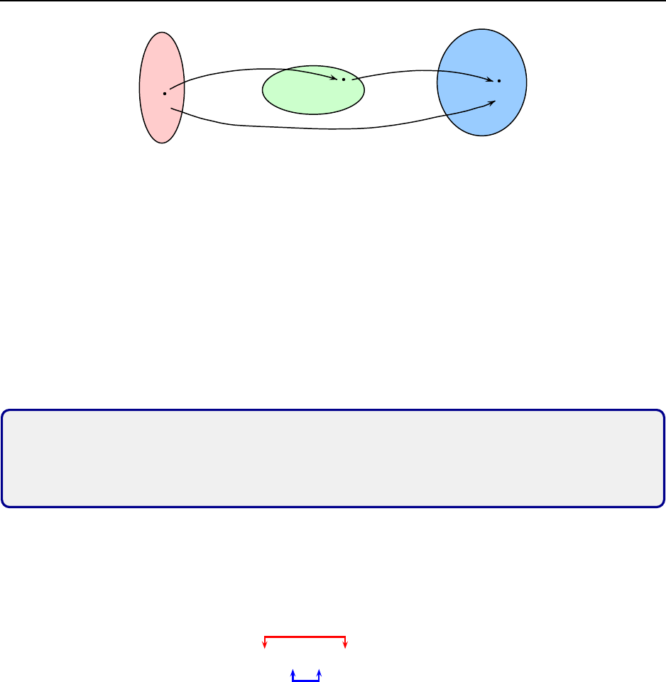
Lecture 9
R
p
R
n
R
m
x
T
B
(x)
T
A
(T
B
(x))
T
B
T
A
(T
A
◦ T
B
)(x)
Figure 9.1: Illustration of the composition of two ma ppings.
Now Be
1
is
Be
1
=
b
1
b
2
··· b
p
e
1
= b
1
.
And similarly Be
i
= b
i
for all i = 1, 2, . . . , p. Therefore,
C =
Ab
1
Ab
2
··· Ab
p
is the standard ma t rix of T
A
◦ T
B
. This computation motivates the following definition.
Definition 9.5: For A ∈ R
m×n
and B ∈ R
n×p
, with B =
b
1
b
2
··· b
p
, we define t he
product AB by the formula
AB =
Ab
1
Ab
2
··· Ab
p
.
The product AB is defined only when the number of columns of A equals the number of
rows o f B. The following diagram is useful for remembering this:
(m × n) · (n × p) → m × p
From our definition of AB, the standard matrix of the composite mapping T
A
◦ T
B
is
C = AB.
In other words, composition of linear mappings corresponds to matrix multiplication.
Example 9.6. For A and B below compute AB and BA.
A =
1 2 −2
1 1 −3
, B =
−4 2 4 −4
−1 −5 −3 3
−4 −4 −3 −1
77

Matrix Algebra
Solution. First AB = [Ab
1
Ab
2
Ab
3
Ab
4
]:
AB =
1 2 −2
1 1 −3
−4 2 4 −4
−1 −5 −3 3
−4 −4 −3 −1
=
2
7
=
2 0
7 9
=
2 0 4
7 9 10
=
2 0 4 4
7 9 10 2
On the other hand, BA is not defined! B has 4 columns and A has 2 rows.
Example 9.7. For A and B below compute AB and BA.
A =
−4 4 3
3 −3 −1
−2 −1 1
, B =
−1 −1 0
−3 0 −2
−2 1 −2
Solution. First AB = [Ab
1
Ab
2
Ab
3
]:
AB =
−4 4 3
3 −3 −1
−2 −1 1
−1 −1 0
−3 0 −2
−2 1 −2
=
−14
8
3
=
−14 7
8 −4
3 3
=
−14 7 −14
8 −4 8
3 3 0
78

Lecture 9
Next BA = [Ba
1
Ba
2
Ba
3
]:
BA =
−1 −1 0
−3 0 −2
−2 1 −2
−4 4 3
3 −3 −1
−2 −1 1
=
1
16
15
=
1 −1
16 −10
15 −9
=
1 −1 −2
16 −10 −11
15 −9 −9
On the other hand:
AB =
−14 7 −14
8 −4 8
3 3 0
Therefore, in general AB 6= BA, i.e., matrix multiplication is not commutative.
An important matrix that arises frequently is the identity matrix I
n
∈ R
n×n
of size
n:
I
n
=
1 0 0 ··· 0
0 1 0 ··· 0
.
.
.
.
.
.
.
.
. ···
.
.
.
0 0 0 ··· 1
You should verify t hat for any A ∈ R
n×n
it holds that AI
n
= I
n
A = A. Below are some
basic algebraic properties of matrix multiplicatio n.
Theorem 9.8: Let A, B, C be matr ices, of appropriate dimensions, and let α be a scalar.
Then
(1) A(BC) = (AB)C
(2) A(B + C) = AB + AC
(3) (B + C)A = BA + CA
(4) α(AB) = (αA)B = A(αB)
(5) I
n
A = AI
n
= A
If A ∈ R
n×n
is a square matrix, the kth power of A is
A
k
= AAA ···A
|
{z }
k times
79

Matrix Algebra
Example 9.9. Compute A
3
if
A =
−2 3
1 0
.
Solution. Compute A
2
:
A
2
=
−2 3
1 0
−2 3
1 0
=
7 −6
−2 3
And then A
3
:
A
3
= A
2
A =
7 −6
−2 3
−2 3
1 0
=
−20 21
7 −6
We could also do:
A
3
= AA
2
=
−2 3
1 0
7 −6
−2 3
=
−20 21
7 −6
.
9.3 Matrix Transpose
We begin with the definition of the transpose of a matrix.
Definition 9.10: Given a matrix A ∈ R
m×n
, the transpose of A is the matrix A
T
whose
ith column is the ith row of A.
If A is m × n then A
T
is n × m. For example, if
A =
0 −1 8 −7 −4
−4 6 −10 −9 6
9 5 −2 −3 5
−8 8 4 7 7
then
A
T
=
0 −4 9 −8
−1 6 5 8
8 −10 −2 4
−7 −9 −3 7
−4 6 5 7
.
Example 9.11. Compute (AB)
T
and B
T
A
T
if
A =
−2 1 0
3 −1 −3
, B =
−2 1 2
−1 −2 0
0 0 −1
.
80

Lecture 9
Solution. Compute AB:
AB =
−2 1 0
3 −1 −3
−2 1 2
−1 −2 0
0 0 −1
=
3 −4 −4
−5 5 9
Next compute B
T
A
T
:
B
T
A
T
=
−2 −1 0
1 −2 0
2 0 −1
−2 3
1 −1
0 −3
=
3 −5
−4 5
−4 9
= (AB)
T
The following theorem summarizes properties of the transpose.
Theorem 9.12: Let A and B be matrices of appropriate sizes. The following ho ld:
(1) (A
T
)
T
= A
(2) (A + B)
T
= A
T
+ B
T
(3) (αA)
T
= αA
T
(4) (AB)
T
= B
T
A
T
A consequence of property (4) is that
(A
1
A
2
. . . A
k
)
T
= A
T
k
A
T
k−1
···A
T
2
A
T
1
and as a special case
(A
k
)
T
= (A
T
)
k
.
Example 9.13. Let T : R
2
→ R
2
be t he linear mapping that first contracts vectors by a
factor of k = 3 and then rotates by an angle θ. What is the standar d matrix A of T?
Solution. Let e
1
= (1, 0) and e
2
= (0, 1) denote the standard unit vectors in R
2
. From
Lecture 8, the standard matrix of T is A =
T(e
1
) T(e
2
)
. Recall that the standard matrix
of a rotation by θ is
cos(θ) −sin(θ)
sin(θ ) cos(θ)
Contracting e
1
by a factor o f k = 3 results in (
1
3
, 0) and then rotation by θ results in
1
3
cos(θ)
1
3
sin(θ)
= T(e
1
).
81

Matrix Algebra
Contracting e
2
by a factor o f k = 3 results in (0,
1
3
) and then rotation by θ results in
−
1
3
sin(θ)
1
3
cos(θ)
= T(e
2
).
Therefore,
A =
T(e
1
) T(e
2
)
=
"
1
3
cos(θ) −
1
3
sin(θ)
1
3
sin(θ)
1
3
cos(θ)
#
On the other hand, the standard matrix corresponding to a contr action by a factor k =
1
3
is
"
1
3
0
0
1
3
#
Therefore,
"
cos(θ) −sin(θ)
sin(θ) cos(θ)
#
|
{z }
rotation
"
1
3
0
0
1
3
#
|
{z }
contraction
=
"
1
3
cos(θ) −
1
3
sin(θ)
1
3
sin(θ)
1
3
cos(θ)
#
= A
After this lecture you should know the following:
• know how to add and multiply matrices
• that matrix multiplicatio n corresponds to compo sition of linear mappings
• the algebraic properties of mat rix multiplication (Theorem
9.8)
• how to compute the transpose of a matrix
• the properties of matrix transposition ( Theorem
9.12)
82

Lecture 10
Lecture 10
Invertibl e Matrices
10.1 Inver se of a Matrix
The inverse of a square matrix A ∈ R
n×n
generalizes the notion of the reciprocal of a non-
zero number a ∈ R. Formally speaking, the inverse of a non-zero number a ∈ R is t he unique
number c ∈ R such that ac = ca = 1. The inverse of a 6= 0, usually denoted by a
−1
=
1
a
, can
be used to solve the equation ax = b:
ax = b ⇒ a
−1
ax = a
−1
b ⇒ x = a
−1
b.
This motivates the fo llowing definition.
Definition 10.1: A mat r ix A ∈ R
n×n
is called invertible if there exists a matrix C ∈
R
n×n
such that AC = I
n
and CA = I
n
.
If A is invertible then can it have more than one inverse? Suppose that there exists C
1
, C
2
such that AC
i
= C
i
A = I
n
. Then
C
2
= C
2
(AC
1
) = (C
2
A)C
1
= I
n
C
1
= C
1
.
Thus, if A is invertible, it can have only one inverse. This motivates the following definition.
Definition 10.2: If A is invertible then we denote the inverse of A by A
−1
. Thus,
AA
−1
= A
−1
A = I
n
.
Example 10.3. Given A and C below, show t ha t C is the inverse of A.
A =
1 −3 0
−1 2 −2
−2 6 1
, C =
−14 −3 −6
−5 −1 −2
2 0 1
83

Invertible Matrices
Solution. Compute AC:
AC =
1 −3 0
−1 2 −2
−2 6 1
−14 −3 −6
−5 −1 −2
2 0 1
=
1 0 0
0 1 0
0 0 1
Compute CA:
CA =
−14 −3 −6
−5 −1 −2
2 0 1
1 −3 0
−1 2 −2
−2 6 1
=
1 0 0
0 1 0
0 0 1
Therefore, by definition C = A
−1
.
Theorem 10.4: Let A ∈ R
n×n
and suppo se that A is invertible. Then for any b ∈ R
n
the matrix equation Ax = b has a unique solution given by A
−1
b.
Proof: Let b ∈ R
n
be arbitrary. Then multiplying the equation Ax = b by A
−1
from the
left we obtain that
A
−1
Ax = A
−1
b
⇒ I
n
x = A
−1
b
⇒ x = A
−1
b.
Therefore, with x = A
−1
b we have that
Ax = A(A
−1
b) = AA
−1
b = I
n
b = b
and t hus x = A
−1
b is a solution. If
˜
x is another solution of the equation, that is, A
˜
x = b,
then mult iplying both sides by A
−1
we o bt ain that
˜
x = A
−1
b. Thus, x =
˜
x.
Example 10.5. Use the result of Example
10.3. to solve the linear system Ax = b if
A =
1 −3 0
−1 2 −2
−2 6 1
, b =
1
−3
−1
.
Solution. We showed in Example
10.3 that
A
−1
=
−14 −3 −6
−5 −1 −2
2 0 1
.
Therefore, the unique solution to the linear system Ax = b is
A
−1
b =
−14 −3 −6
−5 −1 −2
2 0 1
1
−3
−1
=
1
0
1
84

Lecture 10
Verify:
1 −3 0
−1 2 −2
−2 6 1
1
0
1
=
1
−3
−1
The following theorem summarizes the relationship between the matrix inverse and ma-
trix multiplication a nd matrix transpose.
Theorem 10.6: Let A and B be invertible matrices. Then:
(1) The matrix A
−1
is invertible and its inverse is A:
(A
−1
)
−1
= A.
(2) The matrix A B is invertible and its inverse is B
−1
A
−1
:
(AB)
−1
= B
−1
A
−1
.
(3) The matrix A
T
is invertible and its inverse is (A
−1
)
T
:
(A
T
)
−1
= (A
−1
)
T
.
Proof: To prove (2) we compute
(AB)(B
−1
A
−1
) = ABB
−1
A
−1
= AI
n
A
−1
= AA
−1
= I
n
.
To prove
(3) we compute
A
T
(A
−1
)
T
= (A
−1
A)
T
= I
T
n
= I
n
.
10.2 Computing the Inverse of a Matrix
If A ∈ M
n×n
is invertible, how do we find A
−1
? Let A
−1
=
c
1
c
2
··· c
n
and we will
find expressions f or c
i
. First note that AA
−1
=
Ac
1
Ac
2
··· Ac
n
. On the other hand,
we also have AA
−1
= I
n
=
e
1
e
2
··· e
n
. Therefore, we want to find c
1
, c
2
, . . . , c
n
such
that
Ac
1
Ac
2
··· Ac
n
|
{z }
AA
−1
=
e
1
e
2
··· e
n
|
{z }
I
n
.
To find c
i
we therefore need to solve the linear system Ax = e
i
. Here the image vector “b”
is e
i
. To find c
1
we form the augmented matrix
A e
1
and find its RREF:
A e
1
∼
I
n
c
1
.
85

Invertible Matrices
We will need to do this for each c
2
, . . . , c
n
so we might as well form the combined augmented
matrix
A e
1
e
2
··· e
n
and find the RREF all at once:
A e
1
e
2
··· e
n
∼
I
n
c
1
c
2
··· c
n
.
In summary, t o determine if A
−1
exists and to simultaneously compute it, we compute the
RREF of the augmented ma trix
A I
n
,
that is, A augmented with the n × n identity matrix. If the R REF of A is I
n
, that is
A I
n
∼
I
n
c
1
c
2
··· c
n
then
A
−1
=
c
1
c
2
··· c
n
.
If the RREF of A is not I
n
then A is not invertible.
Example 10.7. Find the inverse of A =
1 3
−1 −2
if it exists.
Solution. Form the augmented matrix
A I
2
and row reduce:
A I
2
=
1 3 1 0
−1 −2 0 1
Add rows R
1
and R
2
:
1 3 1 0
−1 −2 0 1
R
1
+R
2
−−−−→
1 3 1 0
0 1 1 1
Perform the operat ion
−3R
2
+R
1
−−−−−→ :
1 3 1 0
0 1 1 1
−3R
2
+R
1
−−−−−→
1 0 −2 −3
0 1 1 1
Thus, rref(A) = I
2
, and therefore A is invertible. The inverse is
A
−1
=
−2 −3
1 1
Verify:
AA
−1
=
1 3
−1 −2
−2 −3
1 1
=
1 0
0 1
.
Example 10.8. Find the inverse of A =
1 0 3
1 1 0
−2 0 −7
if it exists.
86

Lecture 10
Solution. Form the augmented matrix
A I
3
and row reduce:
1 0 3 1 0 0
1 1 0 0 1 0
−2 0 −7 0 0 1
−R
1
+R
2
, 2R
1
+R
2
−−−−−−−−−−→
1 0 3 1 0 0
0 1 −3 −1 1 0
0 0 −1 2 0 1
−R
3
:
1 0 3 1 0 0
0 1 −3 −1 1 0
0 0 −1 2 0 1
−R
3
−−→
1 0 3 1 0 0
0 1 −3 −1 1 0
0 0 1 −2 0 −1
3R
3
+ R
2
and −3R
3
+ R
1
:
1 0 3 1 0 0
0 1 −3 −1 1 0
0 0 1 −2 0 −1
3R
3
+R
2
, −3R
3
+R
1
−−−−−−−−−−−→
1 0 0 7 0 3
0 1 0 −7 1 −3
0 0 1 −2 0 −1
Therefore, rref(A) = I
3
, and therefore A is invertible. The inverse is
A
−1
=
7 0 3
−7 1 −3
−2 0 −1
Verify:
AA
−1
=
1 0 3
1 1 0
−2 0 −7
7 0 3
−7 1 −3
−2 0 −1
=
1 0 0
0 1 0
0 0 1
Example 10.9. Find the inverse of A =
1 0 1
1 1 −2
−2 0 −2
if it exists.
Solution. Form the augmented matrix
A I
3
and row reduce:
1 0 1 1 0 0
1 1 −2 0 1 0
−2 0 −2 0 0 1
−R
1
+R
2
, 2R
1
+R
2
−−−−−−−−−−→
1 0 1 1 0 0
0 1 −3 −1 1 0
0 0 0 2 0 1
We need no t go furt her since the rref(A) is not I
3
(rank(A) = 2 ). Therefore, A is not
invertible.
10.3 Inver tible L inear Mappings
Let T
A
: R
n
→ R
n
be a matrix mapping with standard matrix A a nd suppose that A is
invertible. Let T
A
−1
: R
n
→ R
n
be the matrix mapping with standard matr ix A
−1
. Then
the standard matrix of the composite mapping T
A
−1
◦ T
A
: R
n
→ R
n
is
A
−1
A = I
n
.
87

Invertible Matrices
Therefore, (T
A
−1
◦ T
A
)(x) = I
n
x = x. Let’s unravel (T
A
−1
◦ T
A
)(x) to see this:
(T
A
−1
◦ T
A
)(x) = T
A
−1
(T
A
(x)) = T
A
−1
(Ax) = A
−1
Ax = x.
Similarly, the standard matrix of (T
A
◦T
A
−1
) is also I
n
. Intuitively, the linear mapping T
A
−1
undoes what T
A
does, and conversely. Moreover, since Ax = b always has a solution, T
A
is
ont o. And, because the solution to Ax = b is unique, T
A
is one-to-one.
The following theorem summarizes equivalent conditions for matrix invertibility.
Theorem 10.10: Let A ∈ R
n×n
. The following statements are equivalent:
(a) A is invertible.
(b) A is row equivalent to I
n
, that is, rref(A) = I
n
.
(c) The equation Ax = 0 has only the trivial solution.
(d) The linear transfor ma t ion T
A
(x) = Ax is one-to-one.
(e) The linear transformation T
A
(x) = Ax is onto.
(f) The ma trix equation Ax = b is always solva ble.
(g) The columns o f A span R
n
.
(h) The columns of A are linearly independent.
(i) A
T
is invertible.
Proof: This is a summary of all the statements we have proved about matrices and matrix
mappings specialized to the case of square matrices A ∈ R
n×n
. Note that for non-square
matrices, one-to-one does not imply ontoness, and conversely.
Example 10.11. Without doing any arithmetic, write down the inverse of the dilat ion
matrix
A =
"
3 0
0 5
#
.
Example 10.12. Without doing any arithmetic, write down t he inverse of the rotation
matrix
A =
"
cos(θ) −sin(θ)
sin(θ ) cos(θ)
#
.
After this lecture you should know the following:
• how to compute the inverse o f a matrix
• properties of matrix inversion and matrix multiplication
• relate invertibility of a matrix with properties of t he associated linear mapping (1-1,
ont o)
• the characterizations of invertible matrices Theorem
10.10
88

Lecture 11
Lecture 11
Determinants
11.1 D eterminant s of 2 × 2 and 3 × 3 Matrices
Consider a general 2 × 2 linear system
a
11
x
1
+ a
12
x
2
= b
1
a
21
x
1
+ a
22
x
2
= b
2
.
Using elementary row operations, it can be shown that the solution is
x
1
=
b
1
a
22
− b
2
a
12
a
11
a
22
− a
12
a
21
, x
2
=
b
2
a
11
− b
1
a
21
a
11
a
22
− a
12
a
21
,
provided that a
11
a
22
− a
12
a
21
6= 0. Notice the denominator is the same in bo t h expressions.
The number a
11
a
22
−a
12
a
21
then completely characterizes when a 2 ×2 linear system has a
unique solution. This motivates the following definition.
Definition 11.1: Given a 2 × 2 matrix
A =
a
11
a
12
a
21
a
22
we define the determinant of A as
det A = det
a
11
a
12
a
21
a
22
= a
11
a
22
− a
12
a
21
.
An alternative nota t ion for det A is using vertical ba r s:
det
a
11
a
12
a
21
a
22
=
a
11
a
12
a
21
a
22
.
89

Determinants
Example 11.2. Compute the determinant o f A.
(i) A =
3 −1
8 2
(ii) A =
3 1
−6 −2
(iii) A =
−110 0
568 0
Solution. For (i):
det(A) =
3 −1
8 2
= (3)(2) − (8)(−1) = 14
For (ii):
det(A) =
3 1
−6 −2
= (3)(−2) − (−6)(1) = 0
For (iii):
det(A) =
−110 0
568 0
= (−110)(0) − (56 8)(0) = 0
As in the 2 × 2 case, the solution of a 3 × 3 linear system Ax = b can be shown to be
x
1
=
Numerator
1
D
, x
2
=
Numerator
2
D
, x
3
=
Numerator
3
D
where
D = a
11
(a
22
a
33
− a
23
a
32
) − a
12
(a
21
a
33
− a
23
a
31
) + a
13
(a
21
a
32
− a
22
a
31
).
Notice that the terms of D in the parenthesis a r e determinants of 2 × 2 submatrices of A:
D = a
11
(a
22
a
33
− a
23
a
32
|
{z }
a
22
a
23
a
32
a
33
) − a
12
(a
21
a
33
− a
23
a
31
|
{z }
a
21
a
23
a
31
a
33
) + a
13
(a
21
a
32
− a
22
a
31
|
{z }
a
21
a
22
a
31
a
32
).
Let
A
11
=
a
22
a
23
a
32
a
33
, A
12
=
a
21
a
23
a
31
a
33
, and A
13
=
a
21
a
22
a
31
a
32
.
Then we can write
D = a
11
det(A
11
) − a
12
det(A
12
) + a
13
det(A
13
).
The matrix A
11
=
a
22
a
23
a
32
a
33
is obtained from A by deleting the 1st row and the 1st column:
A =
a
11
a
12
a
13
a
21
a
22
a
23
a
31
a
32
a
33
−→ A
11
=
a
22
a
23
a
32
a
33
.
90

Lecture 11
Similarly, the matrix A
12
=
a
21
a
23
a
31
a
33
is obtained from A by deleting the 1st row and the
2nd column:
A =
a
11
a
12
a
13
a
21
a
22
a
23
a
31
a
32
a
33
−→ A
12
=
a
21
a
23
a
31
a
33
.
Finally, the matrix A
13
=
a
21
a
22
a
31
a
32
is obtained from A by deleting the 1st row and the 3rd
column:
A =
a
11
a
12
a
13
a
21
a
22
a
23
a
31
a
32
a
33
−→
a
21
a
22
a
31
a
32
.
Notice also that the sign in fro nt of the coefficients a
11
, a
12
, and a
13
, alt ernat e. This motivates
the following definition.
Definition 11.3: Let A be a 3 × 3 mat rix. Let A
jk
be the 2 × 2 ma trix obtained from
A by deleting the jth row and kth column. Define the cofactor of a
jk
to be the number
C
jk
= (−1)
j+k
det A
jk
. Define the determinant of A to be
det A = a
11
C
11
+ a
12
C
12
+ a
13
C
13
.
This definition of the determinant is called the expansion of the determinant along the
first row. In the cofactor C
jk
= (−1)
j+k
det A
jk
, the expression (−1)
j+k
will evaluate to
either 1 or −1, depending on whether j + k is even or odd. For example, the cofa cto r of a
12
is
C
12
= (−1)
1+2
det A
12
= −det A
12
and the cofacto r of a
13
is
C
13
= (−1)
1+3
det A
13
= det A
13
.
We can also compute the cofactor of the other entries of A in the obvious way. For example,
the cofactor of a
23
is
C
23
= (−1)
2+3
det A
23
= −det A
23
.
A helpful way to remember the sign (−1)
j+k
of a cofactor is to use the matrix
+ − +
− + −
+ − +
.
This works not just for 3 × 3 matrices but for any square n × n matrix.
Example 11.4. Compute the determinant o f the matrix
A =
4 −2 3
2 3 5
1 0 6
91

Determinants
Solution. From the definition of the determinant
det A = a
11
C
11
+ a
12
C
12
+ a
13
C
13
= (4) det A
11
− (−2) det A
12
+ (3) det A
13
= 4
3 5
0 6
+ 2
2 5
1 6
+ 3
2 3
1 0
= 4(3 · 6 − 5 · 0) + 2(2 · 6 − 1 · 5) + 3(2 · 0 − 1 · 3)
= 72 + 14 − 9
= 77
We can compute the determinant of a matrix A by expanding along any row or column.
For example, the expansion of the determinant for the matrix
A =
a
11
a
12
a
13
a
21
a
22
a
23
a
31
a
32
a
33
along the 3rd row is
det A = a
31
a
12
a
13
a
22
a
23
− a
32
a
11
a
13
a
21
a
23
+ a
33
a
11
a
12
a
21
a
22
.
And along the 2 nd column:
det A = −a
12
a
21
a
23
a
31
a
33
+ a
22
a
11
a
13
a
31
a
33
− a
32
a
11
a
13
a
21
a
23
.
The punchline is that any way yo u choose to expand (row or column) you will get the same
answer. If a particular row or column contains zeros, say ent ry a
jk
, then the computation of
the determinant is simplified if you expand along either row j or column k because a
jk
C
jk
= 0
and we need not compute C
jk
.
Example 11.5. Compute the determinant o f the matrix
A =
4 −2 3
2 3 5
1 0 6
Solution. In Example
11.4, we computed det(A) = 77 by expanding a long the 1st row.
92

Lecture 11
Notice that a
32
= 0. Expanding along the 3rd row:
det A = (1) det A
31
− (0) det A
32
+ (6) det A
33
=
−2 3
3 5
+ 6
4 −2
2 3
= 1(−2 · 5 − 3 · 3) + 6(4 · 3 − ( −2) · 2)
= −19 + 96
= 77
11.2 D eterminant s of n × n Matric es
Using the 3 × 3 case as a guide, we define the determinant of a general n × n matrix as
follows.
Definition 11.6: Let A be a n × n matrix. Let A
jk
be t he (n − 1) × (n − 1) matrix
obtained from A by deleting the jth row and kth column, and let C
jk
= (−1)
j+k
det A
jk
be the (j, k)-cofactor of A. The determinant of A is defined to be
det A = a
11
C
11
+ a
12
C
12
+ ··· + a
1n
C
1n
.
The next theorem tells us that we can compute the determinant by expanding along any
row or column.
Theorem 11.7: Let A be a n × n ma trix. Then det A may be obtained by a cofa cto r
expansion along any row or any column of A:
det A = a
j1
C
j1
+ a
j2
C
j2
+ ··· + a
jn
C
jn
.
We obtain two immediate corollaries.
Corollary 11.8: If A has a row or column containing all zeros then det A = 0.
Proof. If the jth row contains all zeros then a
j1
= a
j2
= ··· = a
jn
= 0:
det A = a
j1
C
j1
+ a
j2
C
j2
+ ··· + a
jn
C
jn
= 0.
93

Determinants
Corollary 11.9: For any square matrix A it holds that det A = det A
T
.
Sketch of the proof. Expanding along the jth row of A is equivalent to expanding along
the jth column of A
T
.
Example 11.10. Compute the determinant o f
A =
1 3 0 −2
1 2 −2 −1
0 0 2 1
−1 −3 1 0
Solution. The third row contains two zeros, so expand along this row:
det A = 0 det A
31
− 0 det A
32
+ 2 det A
33
− det A
34
= 2
1 3 −2
1 2 −1
−1 −3 0
−
1 3 0
1 2 −2
−1 −3 1
= 2
1
2 −1
−3 0
− 3
1 −1
−1 0
− 2
1 2
−1 −3
−
1
2 −2
−3 1
− 3
1 −2
−1 1
= 2((0 − 3) − 3(0 − 1) − 2(−3 + 2) ) − ((2 − 6) − 3(1 − 2))
= 5
Example 11.11. Compute the determinant o f
A =
1 3 0 −2
1 2 −2 −1
0 0 2 1
−1 −3 1 0
94

Lecture 11
Solution. Expanding along the second row:
det A = −det A
21
+ 2 det A
22
− (−2) det A
23
− 1 det A
24
= −
3 0 −2
0 2 1
−3 1 0
+ 2
1 0 −2
0 2 1
−1 1 0
+ 2
1 3 −2
0 0 1
−1 −3 0
−
1 3 0
0 0 2
−1 −3 1
= −1(−3 − 12) + 2(−1 − 4) + 2(0) − (0)
= 5
11.3 Triang ular Matrices
Below we int r oduce a class of matrices for which the determinant computation is t rivial.
Definition 11.12: A square matrix A ∈ R
n×n
is called upper triangular if a
jk
= 0
whenever j > k. In other wo r ds, all the entries of A below the diagonal entries a
ii
are
zero. It is called lower triangular if a
jk
= 0 whenever j < k.
For example, a 4 × 4 upper triangula r matrix takes the form
A =
a
11
a
12
a
13
a
14
0 a
22
a
23
a
24
0 0 a
33
a
34
0 0 0 a
44
Expanding along t he first column, we compute
det A = a
11
a
22
a
23
a
24
0 a
33
a
34
0 0 a
44
= a
11
a
22
a
33
a
34
0 a
44
= a
11
a
22
a
33
a
44
.
The general n × n case is similar and is summarized in the following theorem.
Theorem 11.13: The determinant o f a triangular matr ix is the product of its diagonal
entries.
After this lecture you should know the following:
• how to compute the determinant of any sized matrix
• that the determinant of A is equal to the determinant of A
T
• the determinant of a triangular matrix is the product of its diagonal entries
95

Determinants
96

Lecture 12
Lecture 12
Properti e s of the Determinant
12.1 ERO and Dete r min ants
Recall that for a matrix A ∈ R
n×n
we defined
det A = a
j1
C
j1
+ a
j2
C
j2
+ ··· + a
jn
C
jn
where the number C
jk
= (−1)
j+k
det A
jk
is called the (j, k)-cofactor of A a nd
a
j
=
a
j1
a
j2
··· a
jn
denotes the jth row of A. Notice that
det A =
a
j1
a
j2
··· a
jn
C
j1
C
j2
.
.
.
C
jn
.
If we let c
j
=
C
j1
C
j2
··· C
jn
then
det A = a
j
· c
T
j
.
In this lecture, we will establish properties of the determinant under elementary row opera-
tions and some consequences. The following theorem describes how the determinant behaves
under elementary row operations of Type 1.
Theorem 12.1: Suppose that A ∈ R
n×n
and let B be the matr ix obtained by interchang-
ing two rows of A. Then det B = −det A.
Proof. Consider the 2 × 2 case. Let A =
a
11
a
12
a
21
a
22
and let B =
a
21
a
22
a
11
a
12
. Then
det B = a
12
a
21
− a
11
a
22
= −(a
11
a
22
− a
12
a
21
) = −det A.
The general case is proved by induction.
This theorem leads to the following corollary.
97

Properties of the Determinant
Corollary 12.2: If A ∈ R
n×n
has two rows ( or two columns) that are equal then
det(A) = 0.
Proof. Suppose that A has rows j and k that ar e equal. Let B be the matrix obtained by
interchanging rows j a nd k. Then by the previous theorem det B = −det A. But clearly
B = A, and therefore det B = det A. Therefore, det(A) = −det(A) a nd thus det A = 0.
Now we consider how the determinant behaves under elementary r ow operations of Type
2.
Theorem 12.3: Let A ∈ R
n×n
and let B be t he matr ix obtained by mult iplying a r ow of
A by β. Then det B = β det A.
Proof. Suppose that B is obtained from A by multiplying the jth row by β. The rows of A
and B different from j are equal, and therefore
B
jk
= A
jk
, for k = 1, 2, . . . , n.
In particular, the (j, k) cofactors of A and B are equal. The jth row of B is βa
j
. Then,
expanding det B along t he jth row:
det B = (βa
j
) · c
T
j
= β(a
j
· c
T
j
)
= β det A.
Lastly we consider Type 3 elementary row operations.
Theorem 12.4: Let A ∈ R
n×n
and let B be the matrix obtained from A by adding β
times the kth row to the jth row. Then det B = det A.
Proof. Fo r any matrix A and any row vector r = [r
1
r
2
··· r
n
] the expression
r · c
T
j
= r
1
C
j1
+ r
2
C
j2
+ ··· + r
n
C
jn
is the determinant of the matrix obtained from A by replacing the jth row with the row r.
Therefore, if k 6= j then
a
k
· c
T
j
= 0
98

Lecture 12
since then rows k and j are equal. The jth row of B is b
j
= a
j
+ βa
k
. Therefore, expanding
det B along the jth row:
det B = (a
j
+ βa
k
) · c
T
j
= a
j
· c
T
j
+ β
a
k
· c
T
j
= det A.
Example 12.5. Suppose that A is a 4 × 4 matrix and suppose that det A = 11. If B is
obtained from A by interchanging rows 2 and 4, what is det B?
Solution. Interchanging (or swapping) rows changes the sign of the determinant. Therefore,
det B = −11.
Example 12.6. Suppose that A is a 4 × 4 matrix and suppose that det A = 11. Let
a
1
, a
2
, a
3
, a
4
denote the rows o f A. If B is obtained from A by replacing row a
3
by 3a
1
+ a
3
,
what is det B?
Solution. This is a Type 3 elementary row operation, which preserves the value o f the de-
terminant. Therefore,
det B = 11.
Example 12.7. Suppose that A is a 4 × 4 matrix and suppose that det A = 11. Let
a
1
, a
2
, a
3
, a
4
denote the rows of A. If B is obtained from A by replacing row a
3
by 3a
1
+7a
3
,
what is det B?
Solution. This is not quite a Type 3 elementary row operation because a
3
is multiplied by
7. The third row of B is b
3
= 3a
1
+ 7a
3
. Therefore, expanding det B along the third row
det B = (3a
1
+ 7a
3
) · c
T
3
= 3a
1
· c
T
3
+ 7a
3
· c
T
3
= 7(a
3
· c
T
3
)
= 7 det A
= 77
99

Properties of the Determinant
Example 12.8. Suppose that A is a 4 × 4 matrix and suppose that det A = 11. Let
a
1
, a
2
, a
3
, a
4
denote the rows of A. If B is obtained from A by replacing row a
3
by 4a
1
+5a
2
,
what is det B?
Solution. Again, this is not a Type 3 elementary row operation. The third row of B is
b
3
= 4a
1
+ 5a
2
. Therefore, expanding det B along the third row
det B = (4a
1
+ 5a
2
) · c
T
3
= 4a
1
· c
T
3
+ 5a
2
· c
T
3
= 0 + 0
= 0
12.2 D eterminant s and Invertibility of Matrices
The following theorem char acterizes invertibility of matrices with the determinant.
Theorem 12.9: A square matrix A is invertible if and only if det A 6= 0.
Proof. Beginning with the matrix A, perform elementary row operations and generate a
sequence of matrices A
1
, A
2
, . . . , A
p
such that A
p
is in row echelon form and thus triangular:
A ∼ A
1
∼ A
2
∼ ··· ∼ A
p
.
Thus, matr ix A
i
is obtained from A
i−1
by performing o ne of the elementary row operations.
From Theorems 12.1, 12.3, 12.4, if det A
i−1
6= 0 then det A
i
6= 0. In particular, det A = 0 if
and only if det A
p
= 0. Now, A
p
is triangular and therefore its determinant is the product
of its diagonal entries. If all the diagonal entries are non-zero then det A = det A
p
6= 0. In
this case, A is invertible because there a r e r = n leading entries in A
p
. If a diagonal entry
of A
p
is zero then det A = det A
p
= 0. In this case, A is not invertible because there are
r < n leading entries in A
p
. Therefore, A is invertible if and only if det A 6= 0.
12.3 Pro pe r ties of the Determinant
The following theorem characterizes how the determinant behaves under scalar multiplication
of matrices.
Theorem 12.10: Let A ∈ R
n×n
and let B = βA, that is, B is obtained by multiplying
every entry of A by β. Then det B = β
n
det A.
100

Lecture 12
Proof. Consider the 2 × 2 case:
det(βA) =
βa
11
βa
12
βa
12
βa
22
= βa
11
· βa
22
− βa
12
· βa
21
= β
2
(a
11
a
22
− a
12
a
21
)
= β
2
det A.
Thus, the statement ho lds for 2 × 2 matrices. Consider a 3 × 3 matrix A. Then
det(βA) = βa
11
|βA
11
| − βa
12
|βA
12
| + βa
13
|βA
13
|
= βa
11
β
2
|A
11
| − βa
12
β
2
|A
12
| + βa
13
β
2
|A
13
|
= β
3
(a
11
|A
11
| − a
12
|A
12
| + a
13
|A
13
|)
= β
3
det A.
The general case can be treat ed using mathematical induction on n.
Example 12.11. Suppose that A is a 4 × 4 matrix and suppose that det A = 11. What is
det(3A)?
Solution. We have
det(3A) = 3
4
det A
= 81 · 11
= 891
The following theorem characterizes how the determinant behaves under matrix multi-
plication.
Theorem 12.12: Let A and B be n × n matrices. Then
det(AB) = det(A) det(B).
Corollary 12.13: For any square matrix det(A
k
) = (det A)
k
.
101

Properties of the Determinant
Corollary 12.14: If A is invertible then
det(A
−1
) =
1
det A
.
Proof. From AA
−1
= I
n
we have t hat det(AA
−1
) = 1. But also
det(AA
−1
) = det(A) det(A
−1
).
Therefore
det(A) det(A
−1
) = 1
or equivalently
det A
−1
=
1
det A
.
Example 12.15. Let A, B , C be n × n matrices. Suppo se that det A = 3, det B = 0, and
det C = 7.
(i) Is AC invertible?
(ii) Is AB invertible?
(iii) Is ACB invertible?
Solution. (i): We have det(AC) = det A det C = 3 · 7 = 21. Thus, AC is invertible.
(ii): We have det(AB) = det A det B = 3 · 0 = 0 . Thus, AB is not invertible.
(iii): We have det(ACB) = det A det C det B = 3·7·0 = 0. Thus, ACB is not invertible.
After this lecture you should know the following:
• how the determinant behaves under elementary row operations
• that A is invertible if and o nly if det A 6= 0
• that det(AB) = det(A) det(B)
102
Lecture 13
Lecture 13
Applications of the Determ inant
13.1 The C ofactor Meth od
Recall that for A ∈ R
n×n
we defined
det A = a
j1
C
j1
+ a
j2
C
j2
+ ··· + a
jn
C
jn
where C
jk
= (−1)
j+k
det A
jk
is called the (j, k)-Cofactor of A and
a
j
=
a
j1
a
j2
··· a
jn
is the jth row of A. If c
j
=
C
j1
C
j2
··· C
jn
then
det A =
a
j1
a
j2
··· a
jn
C
j1
C
j2
.
.
.
C
jn
= a
j
· c
T
j
.
Suppose that B is the mat rix obtained from A by r eplacing row a
j
with a distinct row a
k
.
To compute det B expand along its jth row b
j
= a
k
:
det B = a
k
· c
T
j
= 0.
The Cofactor Method is an alternative method to find the inverse of an invertible matrix.
Recall that for any matrix A ∈ R
n×n
, if we expand along the jth row then
det A = a
j
· c
T
j
.
On the other hand, if j 6= k then
a
j
· c
T
k
= 0.
In summary,
a
j
· c
T
k
=
(
det A, if j = k
0, if j 6= k.
103

Applications of the Determinant
Form the Cofactor matrix
Cof(A) =
C
11
C
12
··· C
1n
C
21
C
22
··· C
2n
.
.
.
.
.
. ···
.
.
.
C
n1
C
n2
··· C
nn
=
c
1
c
2
.
.
.
c
n
.
Then,
A(Cof(A))
T
=
a
1
a
2
.
.
.
a
n
c
T
1
c
T
2
··· c
T
n
=
a
1
c
T
1
a
1
c
T
2
··· a
1
c
T
n
a
2
c
T
1
a
2
c
T
2
··· a
2
c
T
n
.
.
.
.
.
.
.
.
.
.
.
.
a
n
c
T
1
a
n
c
T
2
··· a
n
c
T
n
=
det A 0 ··· 0
0 det A ··· 0
.
.
.
.
.
.
.
.
.
.
.
.
0 0 ··· det A
This can be written succinctly as
A(Cof(A))
T
= det(A)I
n
.
Now if det A 6= 0 then we can divide by det A to obtain
A
1
det A
(Cof(A))
T
= I
n
.
This leads to the following formula for the inverse:
A
−1
=
1
det A
(Cof(A))
T
Although this is an explicit and elegant formula for A
−1
, it is computationally intensive,
even for 3 ×3 matrices. However, for the 2 ×2 case it provides a useful formula to compute
104

Lecture 13
the matrix inverse. Indeed, if A =
a b
c d
we have Cof(A) =
d −c
−b a
and therefore
A
−1
=
1
ad − bc
d −b
−c a
.
When does an integer mat rix have an integer inverse? We can a nswer this question
using the Cofactor Method. Let us first be clear about what we mean by an integer matrix.
Definition 13.1: A matrix A ∈ R
m×n
is called an integer matrix if every entry of A is
an integer.
Suppose that A ∈ R
n×n
is an invertible integer matrix. Then det(A) is a non-zero integer
and (Cof(A))
T
is an int eger matrix. If A
−1
is also an integer matrix then det(A
−1
) is also
an integer. Now det(A) det(A
−1
) = 1 thus it must be the case that det(A) = ±1. Suppose
on the other hand that det(A ) = ±1. Then by the Cofactor method
A
−1
=
1
det(A)
(Cof(A))
T
= ±(Cof(A))
T
and therefore A
−1
is also an integer matrix. We have proved the following.
Theorem 13.2: An invertible integer matrix A ∈ R
n×n
has an integer inverse A
−1
if and
only if det A = ±1.
We can use the previous theorem to generate integer matr ices with an integer inverse
as follows. Begin with an upp er triangular matrix M
0
having integer entries and whose
diagonal entries are either 1 or −1. By construction, det(M
0
) = ±1. Perform any sequence
of elementary row operations of Type 1 and Type 3. This generates a sequence of matrices
M
1
, . . . , M
p
whose entries are integers. Moreover,
M
0
∼ M
1
∼ ··· ∼ M
p
.
Therefore,
±1 = det(M) = det(M
1
) = ··· = det(M
p
).
105

Applications of the Determinant
13.2 Cramer’s Rule
The Cofactor method can be used to give an explicit formula for the solution of a linear
system where the coefficient matrix is invertible. The formula is known a s Cramer’s Rule.
To derive this formula, recall that if A is invertible then the solution to Ax = b is x = A
−1
b.
Using the Cofactor method, A
−1
=
1
det A
(Cof(A))
T
, and therefore
x =
1
det A
C
11
C
21
··· C
n1
C
12
C
22
··· C
n2
.
.
.
.
.
.
.
.
.
.
.
.
C
1n
C
2n
··· C
nn
b
1
b
2
.
.
.
b
n
.
Consider the first component x
1
of x:
x
1
=
1
det A
(b
1
C
11
+ b
2
C
21
+ ··· + b
n
C
n1
).
The expression b
1
C
11
+ b
2
C
21
+ ··· + b
n
C
n1
is the expansion of the determinant a long the
first column of the matrix obtained from A by replacing t he first column with b:
det
b
1
a
12
··· a
1n
b
2
a
22
··· a
2n
.
.
.
.
.
.
.
.
.
.
.
.
b
n
a
n2
··· a
nn
= b
1
C
11
+ b
2
C
21
+ ··· + b
n
C
n1
Similarly,
x
2
=
1
det A
(b
1
C
12
+ b
2
C
22
+ ···+ b
n
C
n2
)
and (b
1
C
12
+ b
2
C
22
+ ··· + b
n
C
n2
) is the expansion of the determinant along the second
column of the matrix obtained from A by replacing the second column with b. In summary:
Theorem 13.3: (Cramer’s Rule) Let A ∈ R
n×n
be an invertible matrix. Let b ∈ R
n
and let A
i
be the matr ix obtained from A by replacing the ith column with b. Then the
solution to Ax = b is
x =
1
det A
det A
1
det A
2
.
.
.
det A
n
.
Although this is an explicit and elegant formula for x, it is computat ionally intensive, and
used mainly for theoretical purposes.
106

Lecture 13
13.3 Vo lumes
The volume of the parallelepiped determined by the vectors v
1
, v
2
, v
3
is
Vol(v
1
, v
2
, v
3
) = abs(v
T
1
(v
2
× v
3
)) = abs(det
v
1
v
2
v
3
)
where abs(x) denotes the absolute value of the number x. Let A be an invertible matrix and
let w
1
= Av
1
, w
2
= Av
2
, w
3
= Av
3
. How are Vol(v
1
, v
2
, v
2
) and Vol(w
1
, w
2
, w
2
) related?
Compute:
Vol(w
1
, w
2
, w
3
) = abs(det
w
1
w
2
w
3
)
= abs
det
Av
1
Av
2
Av
3
= abs
det(A
v
1
v
2
v
3
)
= abs
det A · det
v
1
v
2
v
3
= abs(det A) · Vol(v
1
, v
2
, v
3
).
Therefore, the number abs(det A) is the fa cto r by which volume is changed under the linear
transformation with matrix A. In summary:
Theorem 13.4: Suppose that v
1
, v
2
, v
3
are vectors in R
3
that determine a parallelepiped
of non-zero volume. Let A be the matrix of a linear transformation and let w
1
, w
2
, w
3
be
the images of v
1
, v
2
, v
3
under A, respectively. Then
Vol(w
1
, w
2
, w
3
) = abs(det A) · Vol(v
1
, v
2
, v
3
).
Example 13.5. Consider t he data
A =
4 1 −1
2 4 1
1 1 4
, v
1
=
1
−1
0
, v
2
=
0
1
2
, v
3
=
−1
5
1
.
and let w
1
= Av
1
, w
2
= Av
2
, and w
3
= Av
3
. Find the volume of the parallelepiped
spanned by the vectors {w
1
, w
2
, w
3
}.
Solution. We compute:
Vol(v
1
, v
2
, v
3
) = abs(det(
v
1
v
2
v
3
)) = abs(−7) = 7
We compute:
det(A) = 55.
Therefore, the volume of the parallelepiped spanned by the vectors { w
1
, w
2
, w
3
} is
Vol(w
1
, w
2
, w
3
) = abs(55 ) × 7 = 385.
107

Applications of the Determinant
After this lecture you should know the following:
• what the Cofactor Method is
• what Cramer’s Rule is
• the geometric interpretation o f the determinant (volume)
108

Lecture 14
Vector Spaces
14.1 Ve ctor Spaces
When you read/hear the word vector you may immediately think of two points in R
2
(or
R
3
) connected by an arrow. Mathematically speaking, a vector is just an element of a
vector space. This then begs the question: What is a vector space? Roughly speaking,
a vector space is a set of objects that can be added and multiplied by scalars. You
have already worked with several types of vector spaces. Examples of vector spaces that you
have already encountered are:
1. the set R
n
,
2. the set of all n × n matrices,
3. the set of all functions fr om [a, b] to R, and
4. the set of all sequences.
In all of these sets, there is an operation of “addition“ and “multiplication by scalars”. Let’s
formalize then exactly what we mean by a vector space.
Definition 14.1: A vector space is a set V of objects, called vectors, o n which two
operations called addition and scalar multiplication have been defined satisfying the
following properties. If u, v, w are in V and if α, β ∈ R are scalars:
(1) The sum u + v is in V. (closure under addition)
(2) u + v = v + u (addition is commutative)
(3) (u + v) + w = u + (v + w) (addition is associativity)
(4) There is a vector in V called the zero vector, denoted by 0, satisfying v + 0 = v.
(5) For each v there is a vector −v in V such tha t v + (−v) = 0.

Vector Spaces
(6) The scalar multiple of v by α, denoted αv, is in V. (closure under scalar multiplica-
tion)
(7) α(u + v) = αu + αv
(8) (α + β)v = αv + βv
(9) α(βv) = (αβ)v
(10) 1v = v
It can be shown that 0 ·v = 0 for any vector v in V. To better understand the definition of
a vector space, we first consider a few elementary examples.
Example 14.2. Let V be the unit disc in R
2
:
V = {(x, y) ∈ R
2
| x
2
+ y
2
≤ 1}
Is V a vector space?
Solution. The circle is not closed under scalar multiplication. For example, take u = (1, 0) ∈
V and multiply by say α = 2. Then αu = (2, 0) is not in V. Therefore, property (6) of the
definition of a vector space fails, and consequently the unit disc is no t a vector space.
Example 14.3. Let V be the graph of the quadratic function f(x) = x
2
:
V =
n
(x, y) ∈ R
2
| y = x
2
o
.
Is V a vector space?
Solution. The set V is not closed under scalar multiplication. For example, u = ( 1, 1) is a
point in V but 2u = (2, 2) is not. You may also notice that V is no t closed under addition
either. For example, both u = (1, 1) and v = (2, 4) are in V but u + v = (3, 5) and (3, 5) is
not a point on the parabola V. Therefore, the graph of f (x) = x
2
is not a vector space.
110

Lecture 14
Example 14.4. Let V be the graph of the function f(x) = 2x:
V = {(x, y) ∈ R
2
| y = 2x}.
Is V a vector space?
Solution. We will show t ha t V is a vector space. First, we verify that V is closed under
addition. We first note that an arbitr ary point in V can be written as u = (x, 2x). Let then
u = (a, 2a) and v = (b, 2b) be points in V. Then
u + v = (a + b, 2a + 2b) = (a + b, 2(a + b)).
Therefore V is closed under addition. Verify that V is closed under scalar multiplication:
αu = α(a, 2a) = (αa, α2a) = (αa, 2(αa)).
Therefore V is closed under scalar multiplication. There is a zero vector 0 = (0, 0) in V:
u + 0 = (a, 2a) + (0, 0) = (a, 2a).
All the other properties of a vector space can be verified to hold; for example, addition is
commutative and associative in V because addition in R
2
is commutative/associative, etc.
Therefore, the gr aph of the function f (x) = 2x is a vector space.
The following example is important (it will appear frequently) and is our first example
of what we could say is an “a bstract vector space”. To emphasize, a vector space is a set
that comes equipped with an operation of addition and scalar multiplication and these two
operations satisfy t he list of properties above.
Example 14.5. Let V = P
n
[t] be the set of all polynomials in the variable t and of degree
at most n:
P
n
[t] =
n
a
0
+ a
1
t + a
2
t
2
+ ··· + a
n
t
n
| a
0
, a
1
, . . . , a
n
∈ R
o
.
Is V a vector space?
Solution. Let u(t) = u
0
+ u
1
t + ···+ u
n
t
n
and let v(t) = v
0
+ v
1
t + ···+ v
n
t
n
be polynomials
in V. We define the addition of u and v as the new polynomial (u + v) as follows:
(u + v)(t) = u(t) + v(t) = (u
0
+ v
0
) + (u
1
+ v
1
)t + ···+ (u
n
+ v
n
)t
n
.
111

Vector Spaces
Then u + v is a polynomial of degree at most n and thus (u + v ) ∈ P
n
[t], and therefore this
shows that P
n
[t] is closed under addition. Now let α be a scalar, define a new polynomial
(αu) as fo llows:
(αu)(t) = (αu
0
) + (αu
1
)t + ···+ (αu
n
)t
n
Then (α u) is a polynomial of degree at most n and thus (αu) ∈ P
n
[t]; hence, P
n
[t] is closed
under scalar multiplication. The 0 vector in P
n
[t] is the zero po lynomial 0(t) = 0. One can
verify that all other properties of the definition of a vector space also hold; for example,
addition is commutative and associative, etc. Thus P
n
[t] is a vector space.
Example 14.6. Let V = M
m×n
be the set of all m×n matrices. Under the usual operations
of addition of matrices and scalar multiplication, is M
n×m
a vector space?
Solution. Given matrices A, B ∈ M
m×n
and a scalar α, we defined the sum A +B by adding
entry-by-entry, and αA by multiplying each entry of A by α. It is clear that the space
M
m×n
is closed under these two operations. The 0 vector in M
m×n
is t he matrix of size
m × n having all entries equal to zero. It can be verified that all other properties of the
definition of a vector space also hold. Thus, the set M
m×n
is a vector space.
Example 14.7. The n-dimensional Euclidean space V = R
n
under the usual operations of
addition and scalar multiplication is vector space.
Example 14.8. Let V = C[a, b] denote the set of functions with domain [a, b] and co-domain
R that are continuous. Is V a vector space?
14.2 S ubspaces of Vector S paces
Frequently, one encounters a vector space W that is a subset of a larger vector space V. In
this case, we would say that W is a subspace of V. Below is the formal definition.
Definition 14.9: Let V be a vector space. A subset W of V is called a subspace of V
if it satisfies the following properties:
(1) The zero vector of V is also in W.
(2) W is closed under addition, that is, if u and v are in W then u + v is in W.
(3) W is closed under scalar multiplication, that is, if u is in W and α is a scalar then
αu is in W.
Example 14.10. Let W be the graph of the function f(x) = 2x:
W = {(x, y) ∈ R
2
| y = 2x}.
Is W a subspace of V = R
2
?
112

Lecture 14
Solution. If x = 0 then y = 2 · 0 = 0 a nd therefore 0 = (0, 0) is in W. Let u = (a, 2a) and
v = (b, 2b) be elements of W. Then
u + v = (a, 2a) + (b, 2b) = (a + b, 2a + 2b) = (a + b
|{z}
x
, 2 (a + b)
|
{z }
x
).
Because the x and y components of u + v satisfy y = 2x then u + v is inside in W. Thus, W
is closed under addition. Let α be any scalar and let u = (a, 2a) be an element o f W. Then
αu = (αa, α2a) = ( αa
|{z}
x
, 2 (αa)
|
{z}
x
)
Because the x and y components of αu satisfy y = 2x then αu is an element of W, and thus
W is closed under scalar multiplication. All three conditions of a subspace ar e satisfied for
W and therefore W is a subspace of V.
Example 14.11. Let W be the first quadrant in R
2
:
W = {(x, y) ∈ R
2
| x ≥ 0, y ≥ 0}.
Is W a subspace?
Solution. The set W contains the zero vector and the sum of two vectors in W is again in
W; you may want to verify this explicitly a s follows: if u
1
= (x
1
, y
1
) is in W then x
1
≥ 0
and y
1
≥ 0, and similarly if u
2
= ( x
2
, y
2
) is in W then x
2
≥ 0 and y
2
≥ 0. Then the sum
u
1
+u
2
= (x
1
+x
2
, y
1
+y
2
) has components x
1
+y
1
≥ 0 and x
2
+y
2
≥ 0 and therefore u
1
+u
2
is in W. However, W is not closed under scalar multiplication. For example if u = (1, 1)
and α = −1 then α u = (−1, −1) is not in W because the components of αu are clearly not
non-negative.
Example 14.12. Let V = M
n×n
be the vector space of all n × n matrices. We define t he
trace of a mat r ix A ∈ M
n×n
as t he sum of its diagonal entries:
tr(A) = a
11
+ a
22
+ ··· + a
nn
.
Let W be the set of all n × n matrices whose trace is zero:
W = {A ∈ M
n×n
| tr(A) = 0}.
Is W a subspace of V?
Solution. If 0 is the n × n zero matrix then clearly t r(0) = 0, and thus 0 ∈ M
n×n
. Suppose
that A and B are in W. Then necessarily tr(A) = 0 and tr(B) = 0. Consider t he matrix
C = A + B. Then
tr(C) = tr(A + B) = (a
11
+ b
11
) + (a
22
+ b
22
) + ···+ (a
nn
+ b
nn
)
= (a
11
+ ··· + a
nn
) + (b
11
+ ··· + b
nn
)
= tr(A) + tr(B)
= 0
113

Vector Spaces
Therefore, tr(C) = 0 a nd consequently C = A + B ∈ W, in other words, W is closed under
addition. Now let α be a scalar and let C = αA. Then
tr(C) = tr(αA) = (αa
11
) + (αa
22
) + ···+ (αa
nn
) = α tr(A) = 0.
Thus, tr(C ) = 0, that is, C = αA ∈ W, and consequently W is closed under scalar multipli-
cation. Therefore, the set W is a subspace of V.
Example 14.13. Let V = P
n
[t] and consider the subset W of V:
W = {u ∈ P
n
[t] | u
′
(1) = 0}
In other words, W consists of polynomials of degree n in the variable t whose derivative at
t = 1 is zero. Is W a subspace of V?
Solution. The zero polynomial 0(t) = 0 clearly has derivative at t = 1 equal to zero, that is,
0
′
(1) = 0, and thus the zero polynomial is in W. Now suppose that u(t) and v(t) a re two
polynomials in W. Then, u
′
(1) = 0 and also v
′
(1) = 0. To verify whether or no t W is closed
under addition, we must determine whether the sum polynomial ( u + v) ( t) ha s a derivative
at t = 1 equal to zero. From the rules of differentia t ion, we compute
(u + v)
′
(1) = u
′
(1) + v
′
(1) = 0 + 0.
Therefore, the polynomial (u + v) is in W, and thus W is closed under addition. Now let α
be any scalar a nd let u(t) be a polynomial in W. Then u
′
(1) = 0. To determine whether or
not the scalar multiple αu(t) is in W we must determine if αu(t) has a derivative of zero at
t = 1. Using the rules of differentiation, we compute that
(αu)
′
(1) = α u
′
(1) = α · 0 = 0.
Therefore, the polynomial (αu)(t) is in W and thus W is closed under scalar multiplication.
All three properties of a subspace hold for W and therefore W is a subspace of P
n
[t].
Example 14.14. Let V = P
n
[t] and consider the subset W of V:
W = {u ∈ P
n
[t] | u(2) = −1}
In other words, W consists of polynomials of degree n in the variable t whose value t = 2 is
−1. Is W a subspace of V?
Solution. The zero polynomial 0( t) = 0 clearly does not equal −1 at t = 2. Therefore, W
does not contain the zero polynomial and, because all three conditions of a subspace must be
satisfied for W to be a subspace, then W is not a subspace of P
n
[t]. As an exercise, you may
want to investigate whether or not W is closed under addition a nd scalar multiplication.
114

Lecture 14
Example 14.15. A square ma t r ix A is said t o be symmetric if A
T
= A. For example,
here is a 3 × 3 symmetric matrix:
A =
1 2 −3
2 4 5
−3 5 7
Verify for yourself that we do indeed have that A
T
= A. Let W be the set of all symmetric
n × n matrices. Is W a subspace of V = M
n×n
?
Example 14.16. For any vector space V, there are two trivial subspaces in V, namely, V
itself is a subspace of V and the set consisting of the zero vector W = {0} is a subspace of
V.
There is one particular way to generate a subspace o f any given vector space V using the
span of a set of vectors. Recall that we defined the span of a set of vectors in R
n
but we can
define the same notion on a general vector space V.
Definition 14.17: Let V be a vector space and let v
1
, v
2
, . . . , v
p
be vectors in V. The
span of {v
1
, . . . , v
p
} is the set of all linear combinations of v
1
, . . . , v
p
:
span{v
1
, v
2
, . . . , v
p
} =
n
t
1
v
1
+ t
2
v
2
+ ··· + v
p
v
p
| t
1
, t
2
, . . . , t
p
∈ R
o
.
We now show that the span of a set of vectors in V is a subspace of V.
Theorem 14.18: If v
1
, v
2
, . . . , v
p
are vectors in V then span {v
1
, . . . , v
p
} is a subspace of
V.
Solution. Let u = t
1
v
1
+···+t
p
v
p
and w = s
1
v
1
+···+s
p
v
p
be two vectors in span{v
1
, v
2
, . . . , v
p
}.
Then
u + w = (t
1
v
1
+ ··· + t
p
v
p
) + (s
1
v
1
+ ··· + s
p
v
p
) = (t
1
+ s
1
)v
1
+ ··· + (t
p
+ s
p
)v
p
.
Therefore u + w is also in the span of v
1
, . . . , v
p
. Now consider αu:
αu = α(t
1
v
1
+ ··· + t
p
v
p
) = (αt
1
)v
1
+ ··· + (αt
p
)v
p
.
Therefore, αu is in the span of v
1
, . . . , v
p
. Lastly, since 0v
1
+ 0v
2
+ ··· + 0v
p
= 0 then the
zero vector 0 is in t he span of v
1
, v
2
, . . . , v
p
. Therefore, span{v
1
, v
2
, . . . , v
p
} is a subspace
of V.
Given a general subspace W of V, if w
1
, w
2
, . . . , w
p
are vectors in W such tha t
span{w
1
, w
2
, . . . , w
p
} = W
then we say tha t {w
1
, w
2
, . . . , w
p
} is a spanning set of W. Hence, every vector in W can
be written as a linear combination of the vectors w
1
, w
2
, . . . , w
p
.
After this lecture you should know the following:
115

Vector Spaces
• what a vector space/subspace is
• be able to give some examples of vector spaces/subspaces
• that the span of a set of vectors in V is a subspace of V
116

Lecture 15
Lecture 15
Linear Maps
Before we begin this Lecture, we review subspaces. Recall that W is a subspace of a vector
space V if W is a subset of V and
1. the zero vector 0 in V is also in W,
2. for any vectors u, v in W the sum u + v is also in W, and
3. for any vector u in W and a ny scalar α the vector αu is also in W.
In the previous lecture we gave several examples of subspaces. For example, we showed that
a line through the origin in R
2
is a subspace of R
2
and we gave examples of subspaces of
P
n
[t] and M
n×m
. We also showed that if v
1
, . . . , v
p
are vectors in a vector space V then
W = span{v
1
, v
2
, . . . , v
p
}
is a subspace of V.
15.1 Li near Maps on Vector Spaces
In Lecture 7, we defined what it meant for a vector mapping T : R
n
→ R
m
to be a linear
mapping. We now want to introduce linear mappings on general vector spaces; yo u will
notice that the definition is essentially the same but the key point to remember is that the
underlying spaces ar e not R
n
but a general vector space.
Definition 15.1: Let T : V → U be a mapping of vector spaces. Then T is called a linear
mapping if
• for any u, v in V it holds that T(u + v) = T(u) + T(v), and
• for any scalar α and u in V is holds tha t T(αv) = αT(v).
Example 15.2. Let V = M
n×n
be the vector space of n × n matrices and let T : V → V be
the mapping
T(A) = A + A
T
.
117

Linear Maps
Is T is a linear mapping?
Solution. Let A and B be matrices in V. Then using the properties of the transpose and
regrouping we obtain:
T(A + B) = (A + B) + (A + B)
T
= A + B + A
T
+ B
T
= (A + A
T
) + (B + B
T
)
= T(A) + T(B ) .
Similarly, if α is any scalar then
T(αA ) = (αA) + (αA)
T
= αA + αA
T
= α(A + A
T
)
= αT(A).
This proves that T satisfies both conditions of Definition
15.1 and thus T is a linear mapping.
Example 15.3. Let V = M
n×n
be the vector space of n × n matrices, where n ≥ 2 , and let
T : V → R be the mapping
T(A) = det(A )
Is T is a linear mapping?
Solution. If T is a linear ma pping then according t o Definition
15.1, we must have T(A +
B) = det(A + B) = det(A) + det(B) and also T(αA) = αT(A) for any scalar α. Do
these properties a ctually hold though? For example, we know from the properties of the
determinant that det(αA) = α
n
det(A) and therefore it does not hold that T(αA) = αT(A)
unless α = 1. Therefore, T is not a linear ma pping. Also, it does not hold in general that
det(A + B) = det( A) + det(B); in fact it rarely holds. For example, if
A =
2 0
0 1
, B =
−1 1
0 3
then det(A) = 2, det(B) = −3 and therefore det(A ) + det(B) = −1. On the other hand,
A + B =
1 1
0 4
and thus det(A + B) = 4 . Thus, det(A + B) 6= det(A ) + det(B).
Example 15.4. Let V = P
n
[t] be the vector space of polynomials in the variable t of degree
no more than n ≥ 1. Consider the mapping T : V → V define as
T(f(t)) = 2f(t) + f
′
(t).
118

Lecture 15
For example, if f(t) = 3t
6
− t
2
+ 5 then
T(f(t)) = 2f(t) + f
′
(t)
= 2(3t
5
− t
2
+ 5) + (18t
5
− 2t)
= 6t
5
+ 18t
5
− 2t
2
− 2t + 10.
Is T is a linear mapping?
Solution. Let f(t) and g(t) be polynomials of degree no more tha n n ≥ 1. Then
T(f(t) + g( t)) = 2( f (t) + g(t)) + (f(t) + g(t))
′
= 2f(t) + 2g(t) + f
′
(t) + g
′
(t)
= (2f(t) + f
′
(t)) + (2g(t) + g
′
(t))
= T(f(t)) + T(g(t)).
Therefore, T(f (t) + g(t)) = T(f(t)) + T(g(t)). Now let α be any scalar. Then
T(αf (t)) = 2(αf(t)) + (αf(t))
′
= 2αf(t) + αf
′
(t)
= α(2f(t) + f
′
(t))
= αT(f(t)).
Therefore, T(αf(t)) = αT(f(t)). Therefore, T is a linear mapping.
We now introduce two important subsets associated to a linear mapping.
Definition 15.5: Let T : V → U be a linear mapping.
1. The kernel of T is the set of vectors v in the domain V that get mapped to the zero
vector, that is, T(v ) = 0. We denote the kernel of T by ker(T):
ker (T) = {v ∈ V | T(v) = 0}.
2. The range of T is the set of vectors b in the codomain U for which there exists at
least one v in V such that T(v) = b. We denote the r ange of T by Range(T):
Range(T) = {b ∈ U | there exists some v ∈ U such that T(v) = b}.
You may have noticed tha t the definition of the rang e of a linear ma pping on an abstract
vector space is the usual definition of t he range of a function. Not surprisingly, the kernel
and range are subspaces of the doma in and codomain, respectively.
119

Linear Maps
Theorem 15.6: Let T : V → U be a linear mapping. Then ker(T) is a subspace of V and
Range(T) is a subspace of U.
Proof. Suppose that v and u are in ker(T). Then T(v) = 0 and T(u) = 0. Then by linearity
of T it holds that
T(v + u) = T(v) + T(u) = 0 + 0 = 0.
Therefore, since T(u + v) = 0 then u + v is in ker(T). This shows that ker ( T) is closed
under addition. Now suppose that α is any scalar and v is in ker(T). Then T(v) = 0 and
thus by linearity of T it holds that
T(αv) = α T(v) = α0 = 0.
Therefore, since T(αv) = 0 then αv is in ker(T) and this proves that ker(T) is closed under
scalar multiplication. Lastly, by linearity o f T it holds that
T(0) = T( v − v) = T(v) − T(v) = 0
that is, T(0) = 0. Therefore, the zero vector 0 is in ker(T). This proves that ker(T) is a
subspace of V. The proof that Range(T) is a subspace of U is left as an exercise.
Example 15.7. Let V = M
n×n
be the vector space of n × n matrices and let T : V → V be
the mapping
T(A) = A + A
T
.
Describe the kernel of T.
Solution. A mat rix A is in the kernel of T if T(A) = A + A
T
= 0, that is, if A
T
= −A.
Hence,
ker (A) = {A ∈ M
n×n
| A
T
= −A}.
What type of matrix A satisfies A
T
= −A ? For example, consider the case that A is the
2 × 2 matrix
A =
a
11
a
12
a
21
a
22
and A
T
= −A. Then
a
11
a
21
a
12
a
22
=
−a
11
−a
12
−a
21
−a
22
.
Therefore, it must hold that a
11
= −a
11
, a
21
= −a
12
and a
22
= −a
22
. Then necessarily
a
11
= 0 and a
22
= 0 and a
12
can be arbitrary. For example, the matrix
A =
0 7
−7 0
satisfies A
T
= −A. Using a similar computation as above, a 3×3 matrix satisfies A
T
= −A
if A is o f the form
A =
0 a b
−a 0 c
−b −c 0
120

Lecture 15
where a, b, c are arbitr ary constants. In general, a matrix A that satisfies A
T
= −A is called
skew-symmetric.
Example 15.8. Let V be the vector space of differentiable functions on the interval [a, b].
That is, f is an element of V if f : [a, b] → R is differentiable. Describe the kernel of the
linear mapping T : V → V defined as
T(f(x)) = f(x) + f
′
(x).
Solution. A function f is in the kernel of T if T(f(x)) = 0, that is, if f (x) + f
′
(x) = 0.
Equivalently, if f
′
(x) = −f(x). What functions f do you know of satisfy f
′
(x) = −f(x)?
How about f (x) = e
−x
? It is clear that f
′
(x) = −e
−x
= −f(x) and thus f (x) = e
−x
is in
ker (T). How about g(x) = 2e
−x
? We compute t hat g
′
(x) = −2e
−x
= −g(x) and thus g is
also in ker(T). It t urns out that the elements of ker(T) are of the form f(x) = Ce
−x
for a
constant C.
15.2 Null s pace and C olumn space
In the previous section, we introduced the kernel and range of a general linear ma pping
T : V → U. In this section, we consider the particular case of matrix mappings T
A
: R
n
→ R
m
for some m×n matrix A. In this case, v is in the kernel of T
A
if and only if T
A
(v) = Av = 0.
In other words, v ∈ ker(T
A
) if and only if v is a solution to the homogeneous system Ax = 0.
Because the case when T is a mat rix mapping arises so frequently, we give a name to the set
of vectors v such that Av = 0.
Definition 15.9: The null space of a matrix A ∈ M
m×n
, denoted by Null(A) , is the
subset of R
n
consisting of vectors v such that Av = 0. In other words, v ∈ Null(A) if
and only if Av = 0. Using set notation:
Null(A) = {v ∈ R
n
| Av = 0}.
Hence, the following ho lds
ker(T
A
) = Null(A).
Because the kernel of a linear mapping is a subspace we obtain the following.
Theorem 15.10: If A ∈ M
m×n
then Null(A) is a subspace of R
n
.
Hence, by Theorem
15.10, if u and v are two solutions to the linear system Ax = 0 then
αu + βv is also a solution:
A(αu + βv) = αAu + βAv = α · 0 + β · 0 = 0.
121

Linear Maps
Example 15.11. Let V = R
4
and consider t he following subset of V:
W = {(x
1
, x
2
, x
3
, x
4
) ∈ R
4
| 2x
1
− 3x
2
+ x
3
− 7x
4
= 0}.
Is W a subspace of V?
Solution. The set W is the null space of the matrix 1 × 4 matrix A given by
A =
2 −3 1 −7
.
Hence, W = Null(A) and consequently W is a subspace.
From our previous remarks, the null space of a matrix A ∈ M
m×n
is just the solution set
of the homog eneous system Ax = 0. Therefore, one way to explicitly describe the null space
of A is to solve the system Ax = 0 and write the g eneral solution in parametric vector form.
From our previous wo rk on solving linear systems, if the rref(A) has r leading 1 ’s then the
number of parameters in the solution set is d = n − r. Therefore, after performing back
substitution, we will obta in vectors v
1
, . . . , v
d
such that the general solution in parametric
vector form can be written as
x = t
1
v
1
+ t
2
v
2
+ ··· + t
d
v
d
where t
1
, t
2
, . . . , t
d
are arbitrary numbers. Therefore,
Null(A) = span{v
1
, v
2
, . . . , v
d
}.
Hence, the vectors v
1
, v
2
, . . . , v
n
form a spanning set for Null(A ).
Example 15.12. Find a spanning set for the null space of the matrix
A =
−3 6 −1 1 −7
1 −2 2 3 −1
2 −4 5 8 −4
.
Solution. The null space o f A is the solution set of the homogeneous system Ax = 0.
Performing elementary row operations one obtains
A ∼
1 −2 0 −1 3
0 0 1 2 −2
0 0 0 0 0
.
Clearly r = rank(A ) and since n = 5 we will have d = 3 vectors in a spanning set for
Null(A). Letting x
5
= t
1
, and x
4
= t
2
, then from the 2nd row we obtain
x
3
= −2t
2
+ 2t
1
.
Letting x
2
= t
3
, then from the 1st row we obtain
x
1
= 2t
3
+ t
2
− 3t
1
.
122

Lecture 15
Writing the general solution in parametric vector form we obtain
x = t
1
−3
0
2
0
1
+ t
2
1
0
−2
1
0
+ t
3
2
1
0
0
0
Therefore,
Null(A) = span
−3
0
2
0
1
|
{z}
v
1
,
1
0
−2
1
0
|
{z}
v
2
2
1
0
0
0
|
{z}
v
3
You can verify that Av
1
= Av
2
= Av
3
= 0.
Now we consider the range of a matrix mapping T
A
: R
n
→ R
m
. Recall that a vector
b in the co-domain R
m
is in the r ange of T
A
if there exists some vector x in the domain
R
n
such that T
A
(x) = b. Since, T
A
(x) = Ax then Ax = b. Now, if A has columns
A =
v
1
v
2
··· v
n
and x = (x
1
, x
2
, . . . , x
n
) then recall that
Ax = x
1
v
1
+ x
2
v
2
+ ··· + x
n
v
n
and thus Ax = x
1
v
1
+ x
2
v
2
+ ···+ x
n
v
n
= b. Thus, a vector b is in the range of A if it can
be written as a linear combination of the columns v
1
, v
2
, . . . , v
n
of A. This motivates the
following definition.
Definition 15.13: Let A ∈ M
m×n
be a matrix. The span of the columns of A is called
the column space of A. The column space of A is denoted by Col(A). Explicitly, if
A =
v
1
v
2
··· v
n
then
Col(A) = span{v
1
, v
2
, . . . , v
n
}.
In summary, we can write that
Range(T
A
) = Col(A).
and since Range(T
A
) is a subspace of R
m
then so is Col(A).
Theorem 15.14: The column space of a m × n matrix is a subspace of R
m
.
123

Linear Maps
Example 15.15. Let
A =
2 4 −2 1
−2 −5 7 3
3 7 −8 6
, b =
3
−1
3
.
Is b in the column space Col(A) ?
Solution. The vector b is in the column space of A if there exists x ∈ R
4
such that A x = b.
Hence, we must determine if Ax = b has a solution. Perfo rming elementary row operat ions
on the augmented matrix
A b
we o bt ain
A b
∼
2 4 −2 1 3
0 1 −5 −4 −2
0 0 0 17 1
The system is consistent and therefore Ax = b will have a solution. Therefore, b is in
Col(A).
After this lecture you should know the following:
• what the null space of a matrix is and how to compute it
• what the column space o f a matrix is and how to determine if a given vector is in the
column space
• what the range and kernel of a linear mapping is
124

Lecture 16
Linear Independence, Base s, and
Dimension
16.1 Li near In dependence
Roughly speaking, the concept of linear independence evolves ar ound the idea of working
with “efficient” spanning sets for a subspace. For instance, the set of directions
{EAST, NORTH, NORTH-EAST}
are redundant since a to t al displacement in the NORTH-EAST direction can be obtained
by combining individual NORTH and EAST displacements. With these vague statements
out of the way, we introduce the formal definition of what it means for a set of vectors to be
“efficient”.
Definition 16.1: Let V be a vector space and let {v
1
, v
2
, . . . , v
p
} be a set of vectors in
V. Then {v
1
, v
2
, . . . , v
p
} is linearly independent if the only scalars c
1
, c
2
, . . . , c
p
that
satisfy the equation
c
1
v
1
+ c
2
v
2
+ ··· + c
p
v
p
= 0
are the trivial scalars c
1
= c
2
= ··· = c
p
= 0. If the set {v
1
, . . . , v
p
} is not linearly
independent then we say that it is linearly dependent.
We now describe the redundancy in a set of linear dependent vectors. If {v
1
, . . . , v
p
} are
linearly dependent, it follows that there are scalars c
1
, c
2
, . . . , c
p
, at least one of which is
nonzero, such that
c
1
v
1
+ c
2
v
2
+ ··· + c
p
v
p
= 0. (⋆)
For example, suppose that { v
1
, v
2
, v
3
, v
4
} are linearly dependent. Then there are scalars
c
1
, c
2
, c
3
, c
4
, not all of them zero, such that equation (
⋆) holds. Suppose, for the sake of
argument, that c
3
6= 0. Then,
v
3
= −
c
1
c
3
v
1
−
c
2
c
3
v
2
−
c
4
c
3
v
4
.

Linear Independence, Bases, and Dimension
Therefore, when a set of vectors is linearly dependent, it is possible to write one of the vec-
tors as a linear combination of the others. It is in this sense that a set of linearly dependent
vectors are redundant. In fact, if a set of vectors are linearly dependent we can say even
more as the following theorem states.
Theorem 16.2: A set of vectors {v
1
, v
2
, . . . , v
p
}, with v
1
6= 0, is linearly dependent if
and only if some v
j
is a linear combination of the preceding vectors v
1
, . . . , v
j−1
.
Example 16.3. Show that the following set of 2 × 2 matrices is linearly dependent:
A
1
=
1 2
0 −1
, A
2
=
−1 3
1 0
, A
3
=
5 0
−2 −3
.
Solution. It is clear that A
1
and A
2
are linearly independent, i.e., A
1
cannot be written as
a scalar multiple of A
2
, and vice-versa. Since the ( 2, 1) entry of A
1
is zero, the only way to
get the −2 in the (2, 1) entry of A
3
is to multiply A
2
by −2. Similary, since the (2, 2) entry
of A
2
is zero, the only way to get the −3 in the (2, 2) entry of A
3
is to multiply A
1
by 3.
Hence, we suspect that 3A
1
− 2A
2
= A
3
. Verify:
3A
1
− 2A
2
=
3 6
0 −3
−
−2 6
2 0
=
5 0
−2 −3
= A
3
Therefore, 3A
1
− 2A
2
− A
3
= 0 and thus we have f ound scalars c
1
, c
2
, c
3
not all zero such
that c
1
A
1
+ c
2
A
2
+ c
3
A
3
= 0.
16.2 B as es
We now introduce the impo rtant concept of a basis. Given a set of vectors {v
1
, . . . , v
p−1
, v
p
}
in V, we showed that W = span{v
1
, v
2
, . . . , v
p
} is a subspace of V. If say v
p
is linearly
dependent on v
1
, v
2
, . . . , v
p−1
then we can remove v
p
and the smaller set { v
1
, . . . , v
p−1
} still
spans all of W:
W = span{v
1
, v
2
, . . . , v
p−1
, v
p
} = span{v
1
, . . . , v
p−1
}.
Intuitively, v
p
does not provide an independent “direction” in generating W. If some other
vector v
j
is linearly dependent on v
1
, . . . , v
p−1
then we can remove v
j
and the resulting
smaller set o f vectors still spans W. We can continue removing vectors until we o btain a
minimal set of vectors that are linearly independent and still span W. The following remarks
motivate the following important definition.
Definition 16.4: Let W be a subspace of a vector space V. A set of vectors B = {v
1
, . . . , v
k
}
in W is said to be a basis fo r W if
(a) the set B spans all of W, that is, W = span{v
1
, . . . , v
k
}, and
126

Lecture 16
(b) the set B is linearly independent.
A basis is therefore a minimal spanning set for a subspace. Indeed, if B = {v
1
, . . . , v
p
}
is a basis for W and we remove say v
p
, then
˜
B = {v
1
, . . . , v
p−1
} cannot be a basis for W.
Why? If B = {v
1
, . . . , v
p
} is a basis then it is linearly independent and therefore v
p
cannot
be written as a linear combination of the others. In other words, v
p
∈ W is not in the span of
˜
B = {v
1
, . . . , v
p−1
} and therefore
˜
B is not a basis for W because a basis must be a spanning
set. If, on the other hand, we start with a basis B = {v
1
, . . . , v
p
} for W and we add a new
vector u from W then
˜
B = {v
1
, . . . , v
p
, u} is not a basis fo r W. Why? We still have that
span
˜
B = W but now
˜
B is not linearly independent. Indeed, because B = {v
1
, . . . , v
p
} is a
basis for W, the vector u can be written as a linear combination of {v
1
, . . . , v
p
}, and thus
˜
B
is not linearly independent.
Example 16.5. Show that the standard unit vectors form a basis for V = R
3
:
e
1
=
1
0
0
, e
2
=
0
1
0
, e
3
=
0
0
1
Solution. Any vector x ∈ R
3
can be written as a linear combination of e
1
, e
2
, e
3
:
x =
x
1
x
2
x
3
= x
1
1
0
0
+ x
2
0
1
0
+ x
3
0
0
1
= x
1
e
1
+ x
2
e
2
+ x
3
e
3
Therefore, span{e
1
, e
2
, e
3
} = R
3
. The set B = {e
1
, e
2
, e
3
} is linearly independent. Indeed, if
there are scalars c
1
, c
2
, c
3
such that
c
1
e
1
+ c
2
e
2
+ c
3
e
3
= 0
then clearly they must all be zero, c
1
= c
2
= c
3
= 0. Therefore, by definition, B = {e
1
, e
2
, e
3
}
is a basis for R
3
. This basis is called the standard basis for R
3
. Analogous arguments hold
for {e
1
, e
2
, . . . , e
n
} in R
n
.
Example 16.6. Is B = {v
1
, v
2
, v
3
} a basis for R
3
?
v
1
=
2
0
−4
, v
2
=
−4
−2
8
, v
3
=
4
−6
−6
Solution. Form the matrix A = [v
1
v
2
v
3
] and row reduce:
A ∼
1 0 0
0 1 0
0 0 1
127

Linear Independence, Bases, and Dimension
Therefore, the only solution to Ax = 0 is the trivial solution. Therefore, B is linearly inde-
pendent. Moreover, for any b ∈ R
3
, the augmented matrix
A b
is consistent. Therefore,
the columns of A span all of R
3
:
Col(A) = span{v
1
, v
2
, v
3
} = R
3
.
Therefore, B is a basis for R
3
.
Example 16.7. In V = R
4
, consider the vectors
v
1
=
1
3
0
−2
, v
2
=
2
−1
−2
1
, v
3
=
−1
4
2
−3
.
Let W = span{v
1
, v
2
, v
3
}. Is B = {v
1
, v
2
, v
3
} a basis for W?
Solution. By definition, B is a spanning set for W, so we need only determine if B is linearly
independent. Form the matrix, A = [v
1
v
2
v
3
] and row reduce to obtain
A ∼
1 0 1
0 1 −1
0 0 0
0 0 0
Hence, rank(A) = 2 and t hus B is linearly dependent. Notice v
1
− v
2
= v
3
. Therefore, B is
not a basis of W.
Example 16.8. Find a basis for the vector space o f 2 × 2 matrices.
Example 16.9. Recall that a n × n is skew-symmetric A if A
T
= −A. We proved that
the set of n × n matrices is a subspace. Find a basis for the set of 3 × 3 skew-symmetric
matrices.
16.3 D i mension of a Vector Space
The following theorem will lead to the definition of the dimension of a vector space.
Theorem 16.10: Let V be a vector space. Then all bases of V have the same number of
vectors.
Proof: We will prove the theorem for the case that V = R
n
. We already know that the
standard unit vectors {e
1
, e
2
, . . . , e
n
} is a basis of R
n
. L et {u
1
, u
2
, . . . , u
p
} be no nzero vec-
tors in R
n
and suppose first that p > n. In Lecture 6, Theorem
6.7, we proved that any set
of vectors in R
n
containing more than n vectors is automatically linearly dependent. The
reason is that the RREF of A =
u
1
u
2
··· u
p
will contain at most r = n leading ones,
128

Lecture 16
and therefore d = p − n > 0. Therefore, t he solutio n set of Ax = 0 contains non-t rivial
solutions. On the other hand, suppose instead that p < n. In Lecture 4, Theorem
4.11, we
proved that a set of vectors { u
1
, . . . , u
p
} in R
n
spans R
n
if and only if the RREF of A has
exactly r = n leading ones. The largest possible value of r is r = p < n. Therefore, if p < n
then {u
1
, u
2
, . . . , u
p
} cannot be a basis for R
n
. Thus, in either case (p > n or p < n), the set
{u
1
, u
2
, . . . , u
p
} cannot be a basis for R
n
. Hence, any basis in R
n
must conta in n vectors.
The previous theorem does not say that every set {v
1
, v
2
, . . . , v
n
} of nonzero vectors in
R
n
containing n vectors is automatically a basis for R
n
. For example,
v
1
=
1
0
0
, v
2
=
0
1
0
, v
3
=
2
3
0
do not form a basis for R
3
because
x =
0
0
1
is not in the span of {v
1
, v
2
, v
3
}. All that we can say is that a set of vectors in R
n
containing
fewer or more than n vectors is automatically not a basis for R
n
. From Theorem
16.10, any
basis in R
n
must have exactly n vectors. In fact, on a general abstract vector space V, if
{v
1
, v
2
, . . . , v
n
} is a basis for V then any other basis for V must have exactly n vectors also.
Because of this result, we can make the following definition.
Definition 16.11: Let V be a vector space. The dimension of V, denoted dim V, is the
number of vectors in any basis of V. The dimension of the trivial vector space V = {0} is
defined to be zero.
There is one subtle issue we are sweeping under the rug: Does every vector space have a
basis? The answer is yes but we will not prove this result here.
Moving on, suppose that we have a set B = {v
1
, v
2
, . . . , v
n
} in R
n
containing exactly n
vectors. For B = {v
1
, v
2
, . . . , v
n
} to be a ba sis of R
n
, the set B must be linearly independent
and span B = R
n
. In fact, it can b e shown that if B is linearly independent then the spanning
condition span B = R
n
is automatically satisfied, and vice-versa. For example, say the vec-
tors {v
1
, v
2
, . . . , v
n
} in R
n
are linearly independent, a nd put A = [v
1
v
2
··· v
n
]. Then A
−1
exists and therefore Ax = b is always solvable. Hence, Col(A) = span {v
1
, v
2
, . . . , v
n
} = R
n
.
In summary, we have the following theorem.
Theorem 16.12: Let B = {v
1
, . . . , v
n
} be vectors in R
n
. If B is linearly independent
then B is a basis fo r R
n
. Or if span{v
1
, v
2
, . . . , v
n
} = R
n
then B is a basis fo r R
n
.
129

Linear Independence, Bases, and Dimension
Example 16.13. Do the columns of the matrix A form a basis for R
4
?
A =
2 3 3 −2
4 7 8 −6
0 0 1 0
−4 −6 −6 3
Solution. Let v
1
, v
2
, v
3
, v
4
denote the columns of A. Since we have n = 4 vectors in R
n
, we
need only check that they are linearly independent. Compute
det A = −2 6= 0
Hence, rank(A) = 4 and thus the columns of A are linearly independent. Therefore, the
vectors v
1
, v
2
, v
3
, v
4
form a basis fo r R
4
.
A subspace W of a vector space V is a vector space in its own right, and therefore also
has dimension. By definition, if B = {v
1
, . . . , v
k
} is a linearly independent set in W and
span{v
1
, . . . , v
k
} = W, then B is a basis for W and in this case the dimension o f W is k.
Since an n-dimensional vector space V requires exactly n vectors in any basis, then if W is
a strict subspace of V then
dim W < dim V.
As an example, in V = R
3
subspaces can be classified by dimension:
1. The zero dimensional subspace in R
3
is W = {0}.
2. The one dimensional subspaces in R
3
are lines t hrough the origin. These are spanned
by a single non- zero vector.
3. The two dimensional subspaces in R
3
are planes through t he origin. These are spanned
by two linearly independent vectors.
4. The only three dimensional subspace in R
3
is R
3
itself. Any set {v
1
, v
2
, v
3
} in R
3
that
is linearly independent is a basis for R
3
.
Example 16.14. Find a basis for Null(A) and the dim Null(A) if
A =
−2 4 −2 −4
2 −6 −3 1
−3 8 2 −3
.
Solution. By definition, the Null(A) is the solution set of the homogeneous system Ax = 0.
Row reducing we obtain
A ∼
1 0 6 5
0 1 5/2 3/2
0 0 0 0
130

Lecture 16
The general solution to Ax = 0 in parametric for m is
x = t
−5
−3/2
0
1
+ s
−6
−5/2
1
0
= tv
1
+ sv
2
By construction, the vectors
v
1
=
−5
−3/2
0
1
, v
2
=
−6
−5/2
1
0
span the null space (A) and they are linearly independent. Therefore, B = {v
1
, v
2
} is a
basis for Null(A) and therefore dim Null(A) = 2 . In general, the dimension of the Null(A)
is the number of f ree parameters in the solutio n set of the system Ax = 0, that is,
dim Null(A) = d = n − rank(A)
Example 16.15. Find a basis for Col(A) and the dim Col(A) if
A =
1 2 3 −4 8
1 2 0 2 8
2 4 −3 10 9
3 6 0 6 9
.
Solution. By definition, the column space of A is the span of the columns of A, which we
denote by A = [v
1
v
2
v
3
v
4
v
5
]. Thus, to find a basis for Col(A), by trial and error we could
determine the largest subset of the columns of A that are linearly independent. For example,
first we determine if {v
1
, v
2
} is linearly independent. If yes, then add v
3
and determine if
{v
1
, v
2
, v
3
} is linearly independent. If {v
1
, v
2
} is not linearly independent then discard v
2
and determine if {v
1
, v
3
} is linearly independent. We continue this process until we have
determined the largest subset of the columns of A that is linearly independent, and this will
yield a basis for Col(A). Instead, we can use the fact that ma t rices that are r ow equivalent
induce the same solution set for the associated homogeneous system. Hence, let B be the
RREF of A:
B = rref(A) =
1 2 0 2 0
0 0 1 −2 0
0 0 0 0 1
0 0 0 0 0
131

Linear Independence, Bases, and Dimension
By inspection, the columns b
1
, b
3
, b
5
of B are linearly independent. It is easy to see that
b
2
= 2b
1
and b
4
= 2b
1
− 2b
3
. These same linear relatio ns hold for the columns of A :
A =
1 2 3 −4 8
1 2 0 2 8
2 4 −3 10 9
3 6 0 6 9
By inspection, v
2
= 2v
1
and v
4
= 2v
1
− 2v
3
. Thus, because b
1
, b
3
, b
5
are linearly inde-
pendent columns of B =rref(A), then v
1
, v
3
, v
5
are linearly independent columns of A.
Therefore, we have
Col(A) = span{v
1
, v
3
, v
5
} = span
1
1
2
3
,
3
0
−3
0
,
8
8
9
9
and consequently dim Col(A) = 3. This procedure wor ks in general: To find a basis
for the Col(A), row reduce A ∼ B until you can determine which columns of B are linearly
independent. The columns of A in t he same po sition as the linearly independent columns
of B form a basis for the Col(A).
WARNING: Do not take the linearly independent columns of B as a basis f or Col(A).
Always go back to the orig ina l matrix A to select the columns.
After this lecture you should know the following:
• what it means for a set to be linearly independent/dependents
• what a basis is (a spanning set that is linearly independent)
• what is the meaning of t he dimension of a vector space
• how to determine if a given set in R
n
is linearly independent
• how to find a basis for the null space and column space o f a matrix A
132

Lecture 17
The Rank Theorem
17.1 The Rank of a Matrix
We now give the definition to the rank of a matr ix.
Definition 17.1: The rank of a matrix A is the dimension of its column space. We will
use rank(A) to denote the rank of A.
Recall that Col(A) = Range(T
A
), and thus the rank of A is the dimension of the range of
the linear mapping T
A
. The range of a ma pping is sometimes called the image.
We now define the nullity of a matrix.
Definition 17.2: The nullity of a matrix A is t he dimension o f its nullspace Null(A).
We will use nullity(A) to denote the nullity of A.
Recall that (A) = ker(T
A
), and thus the nullity of A is the dimension of the kernel of t he
linear mapping T
A
.
The rank and nullity of a matrix are connected via the following fundamental theorem
known as the Rank Theorem.
Theorem 17.3: (Rank Theorem) Let A be a m × n matrix. The rank o f A is the
number of leading 1’s in its RREF. Moreover, the following equation holds:
n = rank(A) + nullity(A).
Proof. A basis f or the column space is obtained by computing rref(A) and identifying the
columns that contain a leading 1 . Each column of A corresponding to a column of rref(A)
with a leading 1 is a basis vector for the column space of A. Therefore, if r is the number
of leading 1’s then r = r ank(A). Now let d = n − r. The number of free parameters in the

The Rank Theorem
solution set of Ax = 0 is d and therefore a basis for Null(A) will contain d vectors, that is,
nullity(A) = d. Therefore,
nullity(A) = n − ra nk(A).
Example 17.4. Find the rank and nullity of the matrix
A =
1 −2 2 3 −6
0 −1 −3 1 1
−2 4 −3 −6 11
.
Solution. Row reduce far enough to identify where the leading entries a r e:
A
2R
1
+R
2
−−−−→
1 −2 2 3 −6
0 −1 −3 1 1
0 0 1 0 −1
There are r = 3 leading entries and therefore rank(A) = 3. The nullity is therefore
nullity(A) = 5 − r ank(A) = 2.
Example 17.5. Find the rank and nullity of the matrix
A =
1 −3 −1
−1 4 2
−1 3 0
.
Solution. Row reduce far enough to identify where the leading entries a r e:
A
R
1
+R
2
,R
1
+R
3
−−−−−−−−→
1 −3 −1
0 1 1
0 0 −1
There are r = 3 leading entries and therefore rank(A) = 3. The nullity is therefore
nullity(A) = 3 − rank(A) = 0. Another way to see that nullity(A) = 0 is as follows. From
the above computation, A is invertible. Therefore, there is only one vector in Null(A) = {0}.
The subspace {0} has dimension zero.
Using the rank and nullity of a ma t rix, we now provide further characterizations of
invertible matrices.
Theorem 17.6: Let A be a n × n matrix. The following statements are equivalent:
(i) The columns of A form a basis for R
n
.
(ii) Col(A) = R
n
(iii) rank(A) = n
(iv) Null(A) = {0}
134

Lecture 17
(v) nullity( A) = 0
(vi) A is an invertible matrix.
After this lecture you should know the following:
• what the rank of a matr ix is and how to compute it
• what the nullity of a matrix is and how to compute it
• the Rank Theorem
135

The Rank Theorem
136
Lecture 18
Coordi nate Systems
18.1 Coordinates
Recall that a basis of a vector space V is a set of vectors B = {v
1
, v
2
, . . . , v
n
} in V such that
1. the set B spans all of V, that is, V = span(B), and
2. the set B is linearly independent.
Hence, if B is a basis for V, each vector x
∗
∈ V can be written as a linear combination of B:
x
∗
= c
1
v
1
+ c
2
v
2
+ ··· + c
n
v
n
.
Moreover, from the definition of linear independence given in Definition 6.1, any vector
x ∈ span(B) can be written in only one way as a linear combinat ion of v
1
, . . . , v
n
. In ot her
words, for the x
∗
above, there does not exist other scalars t
1
, . . . , t
n
such that also
x
∗
= t
1
v
1
+ t
2
v
2
+ ··· + t
n
v
n
.
To see this, suppose that we can write x
∗
in two different ways using B:
x
∗
= c
1
v
1
+ c
2
v
2
+ ··· + c
n
v
n
x
∗
= t
1
v
1
+ t
2
v
2
+ ··· + t
n
v
n
.
Then
0 = x
∗
− x
∗
= (c
1
− t
1
)v
1
+ (c
2
− t
2
)v
2
+ ··· + (c
n
− t
n
)v
n
.
Since B = {v
1
, . . . , v
n
} is linearly independent, the only linear combination of v
1
, . . . , v
n
that gives the zero vector 0 is the trivial linear combination. Therefore, it must be the case
that c
i
−t
i
= 0, o r equivalently that c
i
= t
i
for all i = 1, 2 . . . , n. Thus, there is only one way
to write x
∗
in terms o f B = {v
1
, . . . , v
n
}. Hence, relative to the basis B = {v
1
, v
2
, . . . , v
n
},
the scalars c
1
, c
2
, . . . , c
n
uniquely determine the vector x, and vice-versa.
Our preceding discussion on the unique representation property of vectors in a given basis
leads to the following definition.

Coordinate Systems
Definition 18.1: Let B = {v
1
, . . . , v
n
} be a basis for V and let x ∈ V. The c oordinates
of x relative to the basis B are the unique scalars c
1
, c
2
, . . . , c
n
such that
x = c
1
v
1
+ c
2
v
2
+ ··· + c
n
v
n
.
In vector notation, the B-coordinates of x will be denoted by
[x]
B
=
c
1
c
2
.
.
.
c
n
and we will call [x]
B
the coordinate vector of x relative to B.
The notation [x]
B
indicates that these are coordinates of x with respect to the basis B.
If it is clear what basis we are working with, we will omit the subscript B and simply write
[x] for the coordinates of x relative to B.
Example 18.2. One can verify that
B =
1
1
,
−1
1
is a basis for R
2
. Find the coordina t es of v =
3
1
relative to B.
Solution. Let v
1
= (1, 1) and let v
2
= (−1, 1). By definition, the coordinat es of v with
respect to B are t he scalars c
1
, c
2
such that
v = c
1
v
1
+ c
2
v
2
=
1 −1
1 1
c
1
c
2
If we put P = [v
1
v
2
], and let [v]
B
= (c
1
, c
2
), then we need to solve the linear system
v = P[v]
B
Solving the linear system, one finds that the solution is [v]
B
= (2, −1), and therefore this is
the B-coordinate vector of v, or the coordinates of v, relative to B.
It is clear how the procedure of the previous example can be generalized. Let B =
{v
1
, v
2
, . . . , v
n
} be a basis for R
n
and let v be any vector in R
n
. Put P =
v
1
v
2
··· v
n
.
Then the B-coordinates of v is the unique column vector [v]
B
solving the linear system
Px = v
138

Lecture 18
that is, x = [v]
B
is the unique solution to Px = v. Because v
1
, v
2
, . . . , v
n
are linearly
independent, the solution to P x = v is
[v]
B
= P
−1
v.
We remark that if an inconsistent row arises when you row reduce the augmented matrix
P v
then you have made an erro r in your row reduction algorithm. In summary, to find
coordinates with respect to a basis B in R
n
, we need to solve a square linear system.
Example 18.3. Let
v
1
=
3
6
2
, v
2
=
−1
0
1
, x =
3
12
7
and let B = {v
1
, v
2
}. One can show that B is linearly independent and therefore a basis for
W = span{v
1
, v
2
}. Determine if x is in W, and if so, find the coordinate vector of x relative
to B.
Solution. By definition, x is in W = span{v
1
, v
2
} if we can write x as a linear combination
of v
1
, v
2
:
x = c
1
v
1
+ c
2
v
2
Form the associated augmented matrix and row reduce:
3 −1 3
6 0 12
2 1 7
∼
1 0 2
0 1 3
0 0 0
The system is consistent with solution c
1
= 2 and c
2
= 3. Therefore, x is in W, and t he
B-coordinat es of x are
[x]
B
=
2
3
Example 18.4. What are the coordinates of
v =
3
11
−7
in the standard basis E = {e
1
, e
2
, e
3
}?
Solution. Clearly,
v =
3
11
−7
= 3
1
0
0
+ 11
0
1
0
− 7
0
0
1
139

Coordinate Systems
Therefore, the coordinate vector of v relative to {e
1
, e
2
, e
3
} is
[v]
E
=
3
11
−7
Example 18.5. Let P
3
[t] be the vector space of polynomials of degree at most 3.
(i) Show that B = {1, t, t
2
, t
3
} is a basis for P
3
[t].
(ii) Find the coordinates of v(t) = 3 − t
2
− 7t
3
relative to B.
Solution. The set B = {1, t, t
2
, t
3
} is a spanning set for P
3
[t]. Indeed, any po lynomial
u(t) = c
0
+ c
1
t + c
2
t
2
+ c
3
t
3
is clearly a linear combination of 1, t, t
2
, t
3
. Is B linearly
independent? Suppose that there exists scalars c
0
, c
1
, c
2
, c
3
such that
c
0
+ c
1
t + c
2
t
2
+ c
3
t
3
= 0.
Since the above equality must hold for all values of t, we conclude that c
0
= c
1
= c
2
= c
3
= 0.
Therefore, B is linearly independent, and consequently a basis for P
3
[t]. In the basis B, the
coordinates of v(t) = 3 − t
2
− 7t
3
are
[v(t)]
B
=
3
0
−1
−7
The basis B = {1, t, t
2
, t
3
} is called the standard basis in P
3
[t].
Example 18.6. Show that
B =
1 0
0 0
,
0 1
0 0
,
0 0
1 0
,
0 0
0 1
is a basis for M
2×2
. Find the coordina t es of A =
3 0
−4 −1
relative to B.
Solution. Any matrix M =
m
11
m
12
m
21
m
22
can be written as a linear combination of the ma-
trices in B:
m
11
m
12
m
21
m
22
= m
11
1 0
0 0
+ m
12
0 1
0 0
+ m
21
0 0
1 0
+ m
22
0 0
0 1
If
c
1
1 0
0 0
+ c
2
0 1
0 0
+ c
3
0 0
1 0
+ c
4
0 0
0 1
=
c
1
c
2
c
3
c
4
=
0 0
0 0
140

Lecture 18
then clearly c
1
= c
2
= c
3
= c
4
= 0. Therefore, B is linearly independent, and consequently
a basis for M
2×2
. The coordinates of A =
3 0
−4 −1
in the basis
B =
1 0
0 0
,
0 1
0 0
,
0 0
1 0
,
0 0
0 1
are
[A]
B
=
3
0
−4
−1
The basis B above is the standard basis of M
2×2
.
18.2 Coordinate Mappings
Let B = {v
1
, v
2
, . . . , v
n
} be a ba sis of R
n
and let P = [v
1
v
2
··· v
n
] ∈ M
n×n
. If x ∈ R
n
and
[x]
B
are the B-coordinates of x relative to B then
x = P[x]
B
. (⋆)
Hence, thinking of P : R
n
→ R
n
as a linear mapping, P maps B-coordinat e vectors to
coordinate vectors relative to the standard basis of R
n
. For this reason, we call P the
change-of-coordinates matrix from the basis B to the standard basis in R
n
. If we need
to emphasize that P is constructed from the basis B we will write P
B
instead of just P.
Multiplying equation (⋆) by P
−1
we obtain
P
−1
x = [x]
B
.
Therefore, P
−1
maps coordinate vectors in the standard basis to coordinates relat ive to B.
Example 18.7. The columns of the ma t r ix P form a basis B f or R
3
:
P =
1 3 3
−1 −4 −2
0 0 −1
.
(a) What vector x ∈ R
3
has B-coordinates [x]
B
= (1, 0, −1).
(b) Find the B-coordinates of v = (2, −1, 0).
Solution. The matrix P maps B-coordinates to standard coordinates in R
3
. Therefore,
x = P[x]
B
=
−2
1
1
141

Coordinate Systems
On the other hand, t he inverse matrix P
−1
maps standard coordinates in R
3
to B-coordinates.
One can verify that
P
−1
=
4 3 6
−1 −1 −1
0 0 −1
Therefore, the B coor dina tes of v are
[v]
B
= P
−1
v =
4 3 6
−1 −1 −1
0 0 −1
2
−1
0
=
5
−1
0
When V is an abstract vector space, e.g. P
n
[t] or M
n×n
, the notion of a coordinate
mapping is similar as the case when V = R
n
. If V is an n- dimensional vector space and
B = {v
1
, v
2
, . . . , v
n
} is a basis for V, we define the coordinate mapping P : V → R
n
relative
to B as the mapping
P(v) = [v]
B
.
Example 18.8. Let V = M
2×2
and let B = {A
1
, A
2
, A
3
, A
4
} be the standard basis for
M
2×2
. What is P : M
2×2
→ R
4
?
Solution. Recall,
B = {A
1
, A
2
, A
3
, A
4
} =
1 0
0 0
,
0 1
0 0
,
0 0
1 0
,
0 0
0 1
Then for any A =
a
11
a
12
a
21
a
22
we have
P
a
11
a
12
a
21
a
22
=
a
11
a
12
a
21
a
22
.
18.3 Matrix Represent ation of a Linear Map
Let V and W be vector spaces and let T : V → W be a linear mapping. Then by definition
of a linear mapping, T(v + u) = T(v) + T(u) and T(αv) = αT(v ) for every v, u ∈ V and
α ∈ R. Let B = {v
1
, v
2
, . . . , v
n
} be a basis of V and let γ = {w
1
, w
2
, . . . , w
m
} be a basis of
W. Then for any v ∈ V there exists scalars c
1
, c
2
, . . . , c
n
such that
v = c
1
v
1
+ c
2
v
2
+ ··· + c
n
v
n
142

Lecture 18
and thus [v]
B
= (c
1
, c
2
, . . . , c
n
) are the coordinates of v in the basis B By linearity of the
mapping T we have
T(v) = T(c
1
v
1
+ c
2
v
2
+ ··· + c
n
v
n
)
= c
1
T(v
1
) + c
2
T(v
2
) + ···+ c
n
T(v
n
)
Now each vector T(v
j
) is in W and therefore because γ is a basis of W there are scalars
a
1,j
, a
2,j
, . . . , a
m,j
such that
T(v
j
) = a
1,j
w
1
+ a
2,j
w
2
+ ··· + a
m,j
w
m
In other words,
[T(v
j
)]
γ
= (a
1,j
, a
2,j
, . . . , a
m,j
)
Substituting T(v
j
) = a
1,j
w
1
+ a
2,j
w
2
+ ··· + a
m,j
w
m
for each j = 1, 2, . . . , n into
T(v) = c
1
T(v
1
) + c
2
T(v
2
) + ···+ c
n
T(v
n
)
and then simplifying we get
T(v) =
m
X
i=1
n
X
j=1
c
j
a
i,j
!
w
i
Therefore,
[T(v)]
γ
= A[v]
B
where A is the m × n matrix given by
A =
[T(v
1
)]
γ
[T(v
2
)]
γ
··· [T(v
n
)]
γ
The matrix A is the matrix r epresentation of the linear mapping T in the bases B and γ.
Example 18.9. Consider the vector space V = P
2
[t] of polynomial of degree no more than
two a nd let T : V → V be defined by
T(v(t)) = 4v
′
(t) − 2v(t)
It is straightforward to verify that T is a linear mapping. Let
B = {v
1
, v
2
, v
3
} = {t − 1, 3 + 2t, t
2
+ 1}.
(a) Verify that B is a basis of V.
(b) Find the coordinates of v ( t) = −t
2
+ 3t + 1 in the basis B.
(c) Find the matrix representa t ion o f T in the basis B.
143

Coordinate Systems
Solution. (a) Suppose that there are scalars c
1
, c
2
, c
3
such that
c
1
v
1
+ c
2
v
2
+ c
3
v
3
= 0
Then expanding and then collecting like terms we obtain
c
3
t
2
+ (c
1
+ 2c
2
)t + (−c
1
+ 3c
2
+ c
3
) = 0
Since the above holds for all t ∈ R we must have
c
3
= 0, c
1
+ 2c
2
= 0, −c
1
+ 3c
2
+ c
3
= 0
Solving for c
1
, c
2
, c
3
we obt ain c
1
= 0, c
2
= 0, c
3
= 0. Hence, the only linear combination of
the vectors in B that produces the zero vector is t he trivial linear combination. This proves
by definition that B is linearly independent. Since we already know that dim(P
2
) = 3 and
B contains 3 vectors, then B is a basis for P
2
(b) The coordinates of v(t) = −t
2
+ 3t + 1 are the unique scalars (c
1
, c
2
, c
3
) such that
c
1
v
1
+ c
2
v
2
+ c
3
v
3
= v
In this case the linear system is
c
3
= −1, c
1
+ 2c
2
= 3, −c
1
+ 3c
2
+ c
3
= 1
and solving yields c
1
= 1, c
2
= 1, and c
3
= −1. Hence,
[v]
B
= (1, 1, −1)
(c) The matrix representation A of T is
A =
[T(v
1
)]
B
[T(v
2
)]
B
[T(v
3
)]
B
Now we compute directly that
T(v
1
) = −2t + 6, T(v
2
) = −4t + 2, T(v
3
) = −2t
2
+ 8t − 2
And then one computes that
[T(v
1
)]
B
=
−18/5
4/5
0
, [T(v
2
)]
B
=
−6/5
−2/5
0
, [T(v
3
)]
B
=
24/5
8/5
−2
And therefore
A =
−18/5 −6/5 24/5
4/5 −2/5 8/5
0 0 −2
144

Lecture 18
After this lecture you should know the following:
• what coordinates are (you need a basis)
• how to find coordinates r elat ive to a basis
• the interpretation of the change-of-coordinates matrix as a mapping that transforms
one set of coordinates to another
145

Coordinate Systems
146
Lecture 19
Change of Basis
19.1 Review of Coordinate Mappings on R
n
Let B = {v
1
, . . . , v
n
} be a basis for R
n
and let
P
B
= [v
1
v
2
··· v
n
].
If x ∈ R
n
and [x]
B
is the coordinate vector of x in the basis B then
x = P
B
[x]
B
.
The components of the vector x are the coordinates of x in the standard basis E = {e
1
, . . . , e
n
}.
In other words,
[x]
E
= x.
Therefore,
[x]
E
= P
B
[x]
B
.
We can therefore interpret P
B
as the matrix mapping that maps the B-coordinates of x to
the E-coo r dina t es of x. To make this mor e explicit, we sometimes use the nota t ion
E
P
B
to indicate tha t
E
P
B
maps B-coordinates to E-coordinates:
[x]
E
= (
E
P
B
)[x]
B
.
If we multiply the equation
[x]
E
= (
E
P
B
)[x]
B
on the left by the inverse of
E
P
B
we obtain
(
E
P
B
)
−1
[x]
E
= [x]
B
Hence, the matrix (
E
P
B
)
−1
maps standard coordinates to B-coordina t es, see Figure
19.1. It
is natural t hen to introduce the notation
B
P
E
= (
E
P
B
)
−1

Change of Basis
x
[x]
B
V = R
n
B
P
E
= (
E
P
B
)
−1
Figure 19.1: The matrix
B
P
E
maps E coordinates to B coordinates.
Example 19.1. Let
v
1
=
1
0
0
, v
2
=
−3
4
0
, v
2
=
3
−6
3
, x =
−8
2
3
.
(a) Show that the set of vectors B = {v
1
, v
2
, v
3
} forms a basis for R
n
.
(b) Find the change-of-coor dina t es matrix from B to standard coordinates.
(c) Find the coordinate vector [x]
B
for the given x.
Solution. Let
P
B
=
1 −3 3
0 4 −6
0 0 3
It is clear that det(P
B
) = 12, and therefore v
1
, v
2
, v
3
are linearly independent . Therefore,
B is a basis for R
n
. The matrix P
B
takes B-coordinates to standard coordinates. The
B-coordinat e vector [x]
B
= (c
1
, c
2
, c
3
) is the unique solution to the linear system
x = P
B
[x]
B
Solving the linear system with augmented matrix [P
B
x] we obtain
[x]
B
= (−5, 2, 1)
We verify that [x]
B
= (−5, 2, 1) are indeed the coordinates of x = (−8, 2, 3) in the basis
148

Lecture 19
B = {v
1
, v
2
, v
3
}:
(−5)v
1
+ (2)v
2
+ (1)v
3
= −5
1
0
0
+ 2
−3
4
0
+
3
−6
3
=
−5
0
0
+
−6
8
0
+
3
−6
3
=
−8
2
3
|
{z}
x
19.2 Change of Basis
We saw in the previous section that the matrix
E
P
B
takes as input the B-coo r dina t es [x]
B
of a vector x and returns the coo rdinates of x in the
standard basis. We now consider the situation of dealing with two basis B and C where
neither is assumed to be the standard basis E. Hence let B = {v
1
, v
2
, . . . , v
n
} and let
C = {w
1
, . . . , w
n
} be two basis of R
n
and let
E
P
B
= [v
1
v
2
··· v
n
]
E
P
C
= [w
1
w
2
··· w
n
].
Then if [x]
C
is the coor dina t e vector of x in the basis C then
x = (
E
P
C
)[x]
C
.
How do we transform B-coordinates of x to C-coo r dina t es of x, and vice-versa? To answer
this question, start from the relations
x = (
E
P
B
)[x]
B
x = (
E
P
C
)[x]
C
.
Then
(
E
P
C
)[x]
C
= (
E
P
B
)[x]
B
and because
E
P
C
is invertible we have that
[x]
C
= (
E
P
C
)
−1
(
E
P
B
)[x]
B
.
149

Change of Basis
Hence, the matrix (
E
P
C
)
−1
(
E
P
B
) maps the B-coo r dina tes of x to the C-coo r dina t es of x. For
this reason, it is natural to use the notation (see Figure
19.2)
C
P
B
= (
E
P
C
)
−1
(
E
P
B
).
x
[x]
C
[x]
B
C
P
B
V = R
n
E
P
B
E
P
C
Figure 19.2: The matrix
C
P
B
maps B-coordinates to C-coordina t es.
If we expand (
E
P
C
)
−1
(
E
P
B
) we obtain that
(
E
P
C
)
−1
(
E
P
B
) =
(
E
P
C
)
−1
v
1
(
E
P
C
)
−1
v
2
··· (
E
P
C
)
−1
v
n
.
Therefore, the ith column of (
E
P
C
)
−1
(
E
P
B
), namely
(
E
P
C
)
−1
v
i
,
is the coordinate vector of v
i
in the basis C = {w
1
, w
2
, . . . , w
n
}. To compute
C
P
B
we
augment
E
P
C
and
E
P
B
and row reduce fully:
E
P
C E
P
B
∼
I
n C
P
B
.
Example 19.2. Let
B =
1
−3
,
−2
4
, C =
−7
9
,
−5
7
It can be verified that B = {v
1
, v
2
} and C = {w
1
, w
2
} are bases f or R
2
.
(a) Find the matrix the takes B-coordinates to C-coordinates.
(b) Find the matrix that takes C-coordinates to B-coordinates.
(c) Let x = (0, −2). Find [x]
B
and [x]
C
.
Solution. The matrix
E
P
B
= [v
1
v
2
] maps B-coordinates to standard E-coordinates. The
matrix
E
P
C
= [w
1
w
2
] maps C-coordinates to standard E-coordinates. As we just showed,
the matrix that maps B-coordinates to C-coordinates is
C
P
B
= (
E
P
C
)
−1
(
E
P
B
)
150

Lecture 19
It is straightforward to compute that
(
E
P
C
)
−1
=
"
−7/4 −5/4
9/4 7/4
#
Therefore,
C
P
B
= (
E
P
C
)
−1
(
E
P
B
) =
"
−7/4 −5/4
9/4 7/4
#"
1 −2
−3 4
#
=
"
2 −3/2
−3 5/2
#
To compute
B
P
C
, we can simply invert
C
P
B
. One finds that
(
C
P
B
)
−1
=
5 3
6 4
and therefore
B
P
C
=
5 3
6 4
Given that x = (0, −2), to find [x]
B
we must solve the linear system
E
P
B
[x]
B
= x
Row reducing the augmented matr ix [
E
P
B
x] we obtain
[x]
B
=
2
1
Next, to find [x]
C
we can solve the linear system
E
P
C
[x]
C
= x
Alternatively, since we now know [x]
B
and
C
P
B
has been computed, to find [x]
C
we simply
multiply
C
P
B
by [x]
B
:
[x]
C
=
C
P
B
[x]
B
=
"
2 −3/2
−3 5/2
#"
2
1
#
=
"
5/2
−7/2
#
Let’s verify that [x]
C
=
5/2
−7/2
are indeed the C-coordinates of x =
0
−2
:
E
P
C
[x]
C
=
"
−7 −5
9 7
#"
5/2
−7/2
#
=
"
0
−2
#
.
After this lecture you should know the following:
• how to compute a change of basis matrix
• and how t o use the change of basis ma t r ix to map one set of coordinates into another
151

Change of Basis
152

Lecture 20
Lecture 20
Inner Products and Orthogonality
20.1 In ner Product on R
n
The inner product on R
n
generalizes the notion of the dot product of vectors in R
2
and R
3
that you may are already familiar with.
Definition 20.1: Let u = (u
1
, u
2
, . . . , u
n
) a nd let v = (v
1
, v
2
, . . . , v
n
) be vectors in R
n
.
The inner product of u and v is
u
•
v = u
1
v
1
+ u
2
v
2
+ ··· + u
n
v
n
.
Notice that the inner product u
•
v can be computed as a matrix multiplication as follows:
u
•
v = u
T
v =
u
1
u
2
··· u
n
v
1
v
2
.
.
.
v
n
.
The following theorem summarizes the ba sic algebraic properties of the inner product.
Theorem 20.2: Let u, v, w be vectors in R
n
and let α be a scalar. Then
(a) u
•
v = v
•
u
(b) (u + v)
•
w = u
•
w + v
•
w
(c) (αu)
•
v = α(u
•
v) = u
•
(αv)
(d) u
•
u ≥ 0, a nd u
•
u = 0 if and only if u = 0
153

Inner Products and Orthogonality
Example 20.3. Let u = (2, −5, −1) and let v = (3, 2, −3). Compute u
•
v, v
•
u, u
•
u, a nd
v
•
v.
Solution. By definition:
u
•
v = (2)(3) + (−5)(2) + (1)(−3) = −1
v
•
u = (3)(2) + (2)( −5) + (−3) ( 1) = −1
u
•
u = (2)(2) + (−5)(−5) + (−1)(−1) = 30
v
•
v = (3)(3) + (2)(2) + (−3)(−3) = 2 2.
We now define the length or norm o f a vector in R
n
.
Definition 20.4: The length or norm o f a vector u ∈ R
n
is defined as
kuk =
√
u
•
u =
q
u
2
1
+ u
2
2
+ ··· + u
2
n
.
A vector u ∈ R
n
with norm 1 will be called a unit vector:
kuk = 1.
Below is an important property of the inner product.
Theorem 20.5: Let u ∈ R
n
and let α be a scalar. Then
kαuk = | α|kuk.
Proof. We have
kαuk =
p
(αu)
•
(αu)
=
p
α
2
(u
•
u)
= |α|
√
u
•
u
= |α|kuk.
By Theorem 20.5, any non-zero vector u ∈ R
n
can be scaled to obtain a new unit vector
in the same direction as u. Indeed, suppose that u is non-zero so that kuk 6= 0. Define the
new vector
v =
1
kuk
u
154

Lecture 20
Notice that α =
1
kuk
is just a scalar and thus v is a scalar multiple of u. Then by Theorem 2 0.5
we have that
kv k = kαuk = |α| · k uk =
1
kuk
· kuk = 1
and therefore v is a unit vector, see Figure
20.1. The process of taking a non-zero vector u
and creating t he new vector v =
1
kuk
u is sometimes called normalization of u.
u
v =
1
kuk
u
Figure 20.1: Normalizing a non-zero vector.
Example 20.6. L et u = (2, 3, 6) . Compute kuk and find the unit vector v in the same
direction as u.
Solution. By definition,
kuk =
√
u
•
u =
√
2
2
+ 3
2
+ 6
2
=
√
49 = 7.
Then the unit vector that is in the same direction as u is
v =
1
kuk
u =
1
7
2
3
6
=
2/7
3/7
6/7
Verify that kvk = 1:
kv k =
p
(2/7)
2
+ (3/7)
2
+ (6/7)
2
=
p
4/49 + 9/49 + 36/49 =
p
49/49 =
√
1 = 1.
Now that we have the definition of the length of a vector, we can define the not ion of
distance between two vectors.
Definition 20.7: Let u and v be vectors in R
n
. The distance between u and v is the
length of the vector u − v. We will denote the distance between u and v by d(u, v). In
other words,
d(u, v) = ku − vk .
Example 20.8. Find the distance between u =
3
−2
and v =
7
−9
.
Solution. We compute:
d(u, v) = ku − vk =
p
(3 − 7)
2
+ (−2 + 9)
2
=
√
65.
155

Inner Products and Orthogonality
20.2 Ort hogonality
In the context of vectors in R
2
and R
3
, orthogonality is synonymous with perpendicularity.
Below is the general definition.
Definition 20.9: Two vectors u and v in R
n
are said to be orthogonal if u
•
v = 0.
In R
2
and R
3
, the notion of ort hogonality should be familiar to you. In fa ct, using the
Law of Cosines in R
2
or R
3
, one can prove that
u
•
v = kuk · kvkcos(θ) (20.1)
where θ is the angle between u and v. If θ =
π
2
then clearly u
•
v = 0. In higher dimensions,
i.e., n ≥ 4, we can use equation (
20.1) to define the angle between vectors u and v. In other
words, the angle between any two vectors u and v in R
n
is define to be
θ = arccos
u
•
v
kuk · kvk
.
The general notion of orthogonality in R
n
leads to the following theorem from grade
schoo l.
Theorem 20.10: (Pythagorean Theorem) Two vectors u and v are ortho gonal if and
only if ku + vk
2
= kuk
2
+ kvk
2
.
Solution. First recall that ku + vk =
p
(u + v)
•
(u + v) and therefore
ku + vk
2
= (u + v)
•
(u + v)
= u
•
u + u
•
v + v
•
u + v
•
v
= kuk
2
+ 2(u
•
v) + k vk
2
.
Therefore, ku + vk
2
= kuk
2
+ kvk
2
if and only if u
•
v = 0.
We now introduce o r thogonal sets.
Definition 20.11: A set of vectors {u
1
, u
2
, . . . , u
p
} is said to be an orthogonal set if
any pair of distinct vectors u
i
, u
j
are orthogonal, that is, u
i
•
u
j
= 0 whenever i 6= j.
In the following theorem we prove that orthogonal sets are linearly independent.
156

Lecture 20
Theorem 20.12: Let {u
1
, u
2
, . . . , u
p
} be an orthogonal set of non-zero vectors in R
n
.
Then the set {u
1
, u
2
, . . . , u
p
} is linearly independent. In part icular, if p = n then the set
{u
1
, u
2
, . . . , u
n
} is basis for R
n
.
Solution. Suppose that there are scalars c
1
, c
2
, . . . , c
p
such that
c
1
u
1
+ c
2
u
2
+ ··· + c
p
u
p
= 0.
Ta ke the inner product of u
1
with both sides of the above equation:
c
1
(u
1
•
u
1
) + c
2
(u
2
•
u
1
) + ···+ c
p
(u
p
•
u
1
) = 0
•
u
1
.
Since the set is orthogonal, the left-hand side of t he last equation simplifies to c
1
(u
1
•
u
1
).
The right-hand side simplifies to 0. Hence,
c
1
(u
1
•
u
1
) = 0.
But u
1
•
u
1
= ku
1
k
2
is not zero and therefore the only way t hat c
1
(u
1
•
u
2
) = 0 is if c
1
= 0 .
Repeat t he above steps using u
2
, u
3
, . . . , u
p
and conclude that c
2
= 0, c
3
= 0, . . . , c
p
=
0. Therefore, {u
1
, . . . , u
p
} is linearly independent. If p = n, then the set {u
1
, . . . , u
p
} is
automatically a basis for R
n
.
Example 20.13. Is the set {u
1
, u
2
, u
3
} an orthogonal set?
u
1
=
1
−2
1
, u
2
=
0
1
2
, u
3
=
−5
−2
1
Solution. Compute
u
1
•
u
2
= (1)(0) + (−2)(1) + (1)(2) = 0
u
1
•
u
3
= (1)(−5) + (−2)(−2) + (1)(1) = 0
u
2
•
u
3
= (0)(−5) + (1)(−2) + (2)(1 ) = 0
Therefore, { u
1
, u
2
, u
3
} is an orthogonal set. By Theorem
20.12, the set {u
1
, u
2
, u
3
} is linearly
independent. To verify linear independence, we computed that det(
u
1
u
2
u
3
) = 30,
which is non-zero.
157

Inner Products and Orthogonality
We now introduce o r thonormal sets.
Definition 20.14: A set of vectors {u
1
, u
2
, . . . , u
p
} is said to be an orthonormal set if
it is an ort hogonal set and if each vector u
i
in the set is a unit vector.
Consider the previous orthogonal set in R
3
:
{u
1
, u
2
, u
3
} =
1
−2
1
,
0
1
2
,
−5
−2
1
.
It is not an orthonormal set because none of u
1
, u
2
, u
3
are unit vectors. Explicitly, ku
1
k =
√
6, ku
2
k =
√
5, and ku
3
k =
√
30. However, from an ort hogonal set we can create an
orthonormal set by normalizing each vector. Hence, the set
{v
1
, v
2
, v
3
} =
1/
√
6
−2/
√
6
1/
√
6
,
0
1/
√
5
2/
√
5
,
−5/
√
30
−2/
√
30
1/
√
30
is an ort ho normal set.
20.3 Coordinates in an Orthonormal Basis
As we will see in this section, a basis B = {u
1
, u
2
, . . . , u
n
} o f R
n
that is also an orthonormal
set is highly desirable when performing computations with coordinates. To see why, let x
be any vector in R
n
and suppose we want to find the coordinates of x in the basis B, that is
we seek to find [x]
B
= (c
1
, c
2
, . . . , c
n
). By definition, the coordinates c
1
, c
2
, . . . , c
n
satisfy the
equation
x = c
1
u
1
+ c
2
u
2
+ ··· + c
n
u
n
.
Ta king the inner product of u
1
with both sides of the above equation and using the fact that
u
1
•
u
2
= 0, u
1
•
u
3
= 0, and u
1
•
u
n
= 0, we obtain
u
1
•
x = c
1
(u
1
•
u
1
) = c
1
(1) = c
1
where we also used the fact that u
i
is a unit vector. Thus, c
1
= u
1
•
x! Repeating this
procedure with u
2
, u
3
, . . . , u
n
we obtain the remaining coefficients c
2
, . . . , c
n
:
c
2
= u
2
•
x
c
3
= u
3
•
x
.
.
. =
.
.
.
c
n
= u
n
•
x.
Our previous computat ion proves the following theorem.
158

Lecture 20
Theorem 20.15: Let B = {u
1
, u
2
, . . . , u
n
} be an orthonormal basis for R
n
. The coordi-
nate vector of x in the basis B is
[x]
B
=
u
1
•
x
u
2
•
x
.
.
.
u
n
•
x
.
Hence, computing coordinates with respect to an orthonormal ba sis can be done without
performing any row operations and all we need to do is compute inner products! We make
the important observation that an alternate expression for [x]
B
is
[x]
B
=
u
1
•
x
u
2
•
x
.
.
.
u
n
•
x
=
u
T
1
u
T
2
.
.
.
u
T
n
x = U
T
x
where U = [u
1
u
2
··· u
n
]. On the other hand, recall that by definition [x]
B
satisfies
U[x]
B
= x, and therefore [x]
B
= U
−1
x. If we compar e the two identities
[x]
B
= U
−1
x and [x]
B
= U
T
x
we suspect then that U
−1
= U
T
. This is indeed the case. To see this, let B = {u
1
, u
2
, . . . , u
n
}
be an orthono rmal basis for R
n
and put
U = [u
1
u
2
··· u
n
].
Consider the matrix product U
T
U, and recalling that u
i
•
u
j
= u
T
i
u
j
, we obtain
U
T
U =
u
T
1
u
T
2
.
.
.
u
T
n
u
1
u
2
··· u
n
=
u
T
1
u
1
u
T
1
u
2
··· u
T
1
u
n
u
T
2
u
1
u
T
2
u
2
··· u
T
2
u
n
.
.
.
.
.
.
.
.
.
.
.
.
u
T
n
u
1
u
T
n
u
2
··· u
T
n
u
n
= I
n
.
159

Inner Products and Orthogonality
Therefore,
U
−1
= U
T
.
A matrix U ∈ R
n×n
such that
U
T
U = UU
T
= I
n
is called a orthogonal matrix. Hence, if B = {u
1
, u
2
, . . . , u
n
} is an orthonormal set then
the matrix
U =
u
1
u
2
··· u
n
is an ort ho gonal matrix.
Example 20.16. Consider t he vectors
v
1
=
1
0
1
, v
2
=
−1
4
1
, v
3
=
2
1
−2
, x =
1
2
−1
.
(a) Show that {v
1
, v
2
, v
3
} is an ort hogonal basis for R
3
.
(b) Then, if necessary, normalize the basis vectors v
i
to obtain an orthono r ma l basis B =
{u
1
, u
2
, u
3
} for R
3
.
(c) For the given x find [x]
B
.
Solution. (a) We compute that v
1
•
v
2
= 0, v
1
•
v
3
= 0, and v
2
•
v
3
= 0, a nd thus {v
1
, v
2
, v
3
}
is an orthogonal set. Since orthogonal sets are linearly independent and {v
1
, v
2
, v
3
}
consists of thr ee vectors then {v
1
, v
2
, v
3
} is basis for R
3
.
(b) We compute that kv
1
k =
√
2, kv
2
k =
√
18, and kv
3
k = 3. Then let
u
1
=
1/
√
2
0
1/
√
2
, u
2
=
−1/
√
18
4/
√
18
1/
√
18
, u
3
=
2/3
1/3
−2/3
Then B = {u
1
, u
2
, u
3
} is now an orthono r ma l set and thus since B consists of three
vectors then B is a n o rthonormal basis of R
3
.
(c) Finally, computing coor dina t es in an orthonorma l ba sis is easy:
[x]
B
=
u
1
•
x
u
2
•
x
u
3
•
x
=
0
2/
√
18
5/3
Example 20.17. The standard unit basis
E = {e
1
, e
2
, e
3
} =
1
0
0
,
0
1
0
,
0
0
1
160

Lecture 20
in R
3
is an orthonormal basis. Given any x = (x
1
, x
2
, x
3
), we have [x]
E
= x. On the other
hand, clearly
x
1
= x
•
e
1
x
2
= x
•
e
2
x
3
= x
•
e
3
Example 20.18. (Orthogonal Complements) Let W be a subspace o f R
n
. The orthogonal
complement of W, which we denote by W
⊥
, consists of the vectors in R
n
that are o rthogonal
to every vector in W. Using set notation:
W
⊥
= {u ∈ R
n
: u
•
w = 0 for every w ∈ W}.
(a) Show that W
⊥
is a subspace.
(b) Let w
1
= (0, 1, 1, 0), let w
2
= (1, 0, −1, 0), and let W = span{w
1
, w
2
}. Find a basis for
W
⊥
.
Solution. (a) The vector 0 is orthogonal to every vector in R
n
and therefore it is certainly
orthogonal to every vector in W. Thus, 0 ∈ W
⊥
. Now suppose that u
1
, u
2
are two
vectors in W
⊥
. Then for any vector w ∈ W it holds that
(u
1
+ u
2
)
•
w = u
1
•
w + u
2
•
w = 0 + 0 = 0.
Therefore, u
1
+ u
2
is also orthogona l to w and since w is an arbitrary vector in W then
(u
1
+ u
2
) ∈ W
⊥
. Lastly, let α be any scalar and let u ∈ W
⊥
. Then for any vector w in
W we have that
(αu)
•
w = α(u
•
w ) = α · 0 = 0.
Therefore, αu is orthogonal to w and since w is an arbitrary vector in W then (αu) ∈ W
⊥
.
This proves that W
⊥
is a subspace of R
n
.
(b) A vector u = (u
1
, u
2
, u
3
, u
3
) is in W
⊥
if u
•
w
1
= 0 and u
•
w
2
= 0. In other words, if
u
2
+ u
3
= 0
u
1
− u
3
= 0
This is a linear system for the unknowns u
1
, u
2
, u
3
, u
4
. The general solution to the linear
system is
u = t
1
0
1
0
+ s
0
1
−1
0
.
Therefore, a basis for W
⊥
is {(1, 0, 1, 0), (0, 1, −1, 0)}.
After this lecture you should know the following:
161

Inner Products and Orthogonality
• how to compute inner products, norms, and distances
• how to normalize vectors to unit length
• what orthogonality is and how to check for it
• what an orthogonal and orthonormal basis is
• the advantages of working with ort honormal basis when computing coordina te vectors
162

Lecture 21
Lecture 21
Eigenvalues and Eigenvectors
21.1 Ei genvectors and Eigenvalues
An n ×n matrix A can be thought o f as the linear mapping that takes any arbitrary vector
x ∈ R
n
and outputs a new vector Ax. In some cases, the new output vector Ax is simply
a scalar multiple of the input vector x, that is, there exists a scalar λ such that Ax = λx.
This case is so important that we make the following definition.
Definition 21.1: Let A be a n × n matrix and let v be a non-zero vector. If Av = λv
for some scalar λ then we call the vector v an eigenvector of A and we call the scalar λ
an eigenvalue of A corresponding to v.
Hence, an eigenvector v of A is simply scaled by a scalar λ under multiplication by A.
Eigenvectors are by definition nonzero vectors because A0 is clearly a scalar multiple of 0
and then it is not clear what that the corresponding eigenvalue should be.
Example 21.2. Determine if the given vectors v and u are eigenvectors of A? If yes, find
the eigenvalue of A associated to the eigenvector.
A =
4 −1 6
2 1 6
2 −1 8
, v =
−3
0
1
, u =
−1
2
1
.
Solution. Compute
Av =
4 −1 6
2 1 6
2 −1 8
−3
0
1
=
−6
0
2
= 2
−3
0
1
= 2v
163

Eigenvalues and Eigenvectors
Hence, Av = 2 v and thus v is an eigenvector of A with corresp onding eigenvalue λ = 2. On
the other hand,
Au =
4 −1 6
2 1 6
2 −1 8
−1
2
1
=
0
6
4
.
There is no scalar λ such that
0
6
4
= λ
−1
2
1
.
Therefore, u is not an eigenvector of A.
Example 21.3. Is v an eigenvector of A? If yes, find the eigenvalue of A associated to v:
A =
2 −1 −1
−1 2 −1
−4 2 2
, v =
1
1
1
.
Solution. We compute
Av =
0
0
0
= 0.
Hence, if λ = 0 then λ v = 0 and thus Av = λv. Therefore, v is an eigenvector o f A with
corresponding eigenvalue λ = 0.
How does one find the eigenvectors/eigenvalues of a matrix A? The general procedure
is to first find the eigenvalues of A and then for each eigenvalue find the corresponding
eigenvectors. In this section, however, we will instead suppose that we have already found
the eigenvalues o f A and concern ourselves with finding the associated eigenvectors. Suppose
then that λ is known to be an eigenvalue of A. How do we find an eigenvector v corresponding
to the eigenvalue λ? To answer this question, we note tha t if v is to be an eigenvector of A
with eigenvalue λ then v must satisfy the equation
Av = λv.
We can rewrite this equation as
Av − λv = 0
which, after using the distributive property of matrix multiplication, is equivalent to
(A − λI)v = 0.
The last equation says that if v is to be an eigenvector of A with eigenvalue λ then v must
be in t he null space of A − λI:
v ∈ Null(A − λI).
164

Lecture 21
In summary, if λ is known to be an eigenvalue of A, then to find the eigenvectors corre-
sponding to λ we must solve the homogeneous system
(A − λI)x = 0.
Recall that the null space of any matrix is a subspace and for this reason we call the subspace
Null(A − λI) the eigenspace of A corresponding to λ.
Example 21.4. It is known that λ = 4 is an eigenvalue of
A =
−4 6 3
1 7 9
8 −6 1
.
Find a basis for the eigenspace o f A corresponding to λ = 4.
Solution. First compute
A − 4I =
−4 6 3
1 7 9
8 −6 1
−
4 0 0
0 4 0
0 0 4
=
−8 6 3
1 3 9
8 −6 −3
Find a basis for the null space of A − 4I:
−8 6 3
1 3 9
8 −6 −3
R
1
lR
2
−−−→
1 3 9
−8 6 3
8 −6 −3
1 3 9
−8 6 3
8 −6 −3
8R
1
+R
2
−8R
1
+R
3
−−−−−−→
1 3 9
0 30 75
0 −30 −75
Finally,
1 3 9
0 30 75
0 −30 −75
R
2
+R
3
−−−−→
1 3 9
0 30 75
0 0 0
Hence, the general solution to the homo genous system (A − 4I)x = 0 is
x = t
−3/2
−5/2
1
where t is an arbitrary scalar. Therefore, the eigenspace of A corresponding to λ = 4 is
span
−3/2
−5/2
1
= span
−3
−5
2
= span{v}
and {v} is a basis for the eigenspace. The vector v is of course an eigenvector of A with
eigenvalue λ = 4 and also (of course) any multiple of v is also eigenvector of A with λ = 4.
165

Eigenvalues and Eigenvectors
Example 21.5. It is known that λ = 3 is an eigenvalue of
A =
11 −4 −8
4 1 −4
8 −4 −5
.
Find the eigenspace of A corresponding to λ = 3 .
Solution. First compute
A − 3I =
11 −4 −8
4 1 −4
8 −4 −5
−
3 0 0
0 3 0
0 0 3
=
8 −4 −8
4 −2 −4
8 −4 −8
Now find the null space of A − 3I:
8 −4 −8
4 −2 −4
8 −4 −8
R
1
lR
2
−−−→
4 −2 −4
8 −4 −8
8 −4 −8
4 −2 −4
8 −4 −8
8 −4 −8
−2R
1
+R
2
−2R
1
+R
3
−−−−−−→
4 −2 −4
0 0 0
0 0 0
Hence, any vector in the null space of
A − 3I =
4 −2 −4
0 0 0
0 0 0
can be written as
x = t
1
1
0
1
+ t
2
1
2
0
Therefore, the eigenspace of A corresponding to λ = 3 is
Null(A − 3I) = span{v
1
, v
2
} = span
1
0
1
,
1
2
0
.
The vectors v
1
and v
2
are two linearly independent eigenvectors of A with eigenvalue λ = 3.
Therefore {v
1
, v
2
} is a basis fo r the eigenspace o f A with eigenvalue λ = 3. You can verify
that Av
1
= 3v
1
and Av
2
= 3v
2
.
As shown in the last example, there may exist more than one linearly independent eigen-
vector of A corresponding t o the same eigenvalue, in other words, it is possible that the
dimension o f the eigenspace Null(A − λI) is greater than one. What can be said about the
eigenvectors of A corresponding to different eigenvalues?
166

Lecture 21
Theorem 21.6: Let v
1
, . . . , v
k
be eigenvectors of A corresponding to distinct eigenvalues
λ
1
, . . . , λ
k
of A. Then {v
1
, . . . , v
k
} is a linearly independent set.
Solution. Suppose by contradiction that {v
1
, . . . , v
k
} is linearly dependent and {λ
1
, . . . , λ
k
}
are distinct. Then, one of the eigenvectors v
p+1
that is a linear combination of v
1
, . . . , v
p
,
and {v
1
, . . . , v
p
} is linearly independent:
v
p+1
= c
1
v
1
+ c
2
v
2
+ ··· + c
p
v
p
. (21.1)
Applying A to both sides we obtain
Av
p+1
= c
1
Av
1
+ c
2
Av
2
+ ··· + c
p
Av
p
and since Av
i
= λ
i
v
i
we can simplify this to
λ
p+1
v
p+1
= c
1
λ
1
v
1
+ c
2
λ
2
v
2
+ ··· + c
p
λ
p
v
p
. (21.2)
On the other hand, multiply (
21.1) by λ
p+1
:
λ
p+1
v
p+1
= c
1
λ
p+1
v
1
+ c
2
λ
p+1
v
2
+ ··· + c
p
v
p
λ
p+1
. (21.3)
Now subtract equations (
21.2) and (21.3):
0 = c
1
(λ
1
− λ
p+1
)v
1
+ c
2
(λ
2
− λ
p+1
)v
2
+ ··· + c
p
(λ
p
− λ
p+1
)v
p
.
Now {v
1
, . . . , v
p
} is linearly independent and thus c
i
(λ
i
− λ
p+1
) = 0. But the eigenvalues
{λ
1
, . . . , λ
k
} are all distinct and so we must have c
1
= c
2
= ··· = c
p
= 0. But from (
21.1)
this implies that v
p+1
= 0, which is a contradiction because eigenvectors are by definition
non-zero. This proves t hat {v
1
, v
2
, . . . , v
k
} is a linearly independent set.
Example 21.7. It is known that λ
1
= 1 and λ
2
= −1 are eigenvalues of
A =
−4 6 3
1 7 9
8 −6 1
.
Find bases for the eigenspaces correspo nding to λ
1
and λ
2
and show t hat any two vectors
from these distinct eigenspaces are linearly independent.
Solution. Compute
A − λ
1
I =
−5 6 3
1 6 9
8 −6 0
and one finds that
(A − λ
1
I) = span
−3
−4
3
167

Eigenvalues and Eigenvectors
Hence, v
1
= (−3, −4, 3) is an eigenvector of A with eigenvalue λ
1
= 1 , and {v
1
} f orms a
basis for the corresponding eigenspace. Next, compute
A − λ
2
I =
−4 6 3
1 7 9
8 −6 1
+
1 0 0
0 1 0
0 0 1
=
−3 6 3
1 8 9
8 −6 2
and one finds that
A − λ
2
I = span
−1
−1
1
Hence, v
2
= (−1, −1, 1) is an eigenvector of A with eigenvalue λ
2
= −1, and {v
2
} forms a
basis for the corresponding eigenspace. Now verify that v
1
and v
2
are linearly independent:
v
1
v
2
=
−3 −1
−4 −1
3 1
R
1
+R
3
−−−−→
−3 −1
−4 −1
0 0
The last matrix has rank r = 2, and thus v
1
, v
2
are indeed linearly independent.
21.2 W hen λ = 0 is an eigenvalue
What can we say about A if λ = 0 is an eigenvalue of A? Suppose then that A has eigenvalue
λ = 0. Then by definition, there exists a non-zero vector v such tha t
Av = 0 · v = 0.
In other words, v is in the null space of A. Thus, A is not invertible (Why?).
Theorem 21.8: The matrix A ∈ R
n×n
is invertible if and only if λ = 0 is not an eigenvalue
of A.
In fact, la t er we will see that det (A) is the product of its eigenvalues.
After this lecture you should know the following:
• what eigenvalues are
• what eigenvectors are and how to find them when eigenvalues a re known
• the behavior of a discrete dynamical system when the initial condition is set to an
eigenvector of the system mat r ix
168

Lecture 22
Lecture 22
The Characteristic Polynomi a l
22.1 The C haracteristic Polyn omial of a Matri x
Recall that a number λ is an eigenvalue of A ∈ R
n×n
if there exists a non-zero vector v such
that
Av = λv
or equivalently if v ∈ Null(A − λI). In other words, λ is an eigenvalue of A if and only
if the subspace Null( A − λI) contains a vector other than the zero vector. We know that
any matrix M has a non-trivial null space if and o nly if M is non-invertible if and only if
det(M) = 0. Hence, λ is an eigenvalue of A if and only if λ satisfies det(A −λI) = 0. Let’s
compute the expression det(A − λI) for a generic 2 × 2 matrix:
det(A − λI) =
a
11
− λ a
12
a
21
a
22
− λ
= (a
11
− λ)(a
22
− λ) − a
12
a
22
= λ
2
− (a
11
+ a
22
)λ + a
11
a
22
− a
12
a
22
.
Thus, if A is 2 × 2 then
det(A − λI) = λ
2
− (a
11
+ a
22
)λ + a
11
a
22
− a
12
a
22
is a po lynomial in the variable λ of degree n = 2. This motivates the following definition.
Definition 22.1: Let A be a n × n matrix. The polynomial
p(λ) = det(A − λI )
is called the characteristic polynomial of A.
169

The Characteristic Polynomial
In summary, to find the eigenvalues of A we must find the roots of the characteristic poly-
nomial:
p(λ) = det(A − λI ) .
The f ollowing theorem asserts that what we observed for the case n = 2 is indeed true for
all n.
Theorem 22.2: The characteristic polynomial p(λ) = det(A − λI) of a n × n matrix A
is an nth degree polynomial.
Solution. Recall that for the case n = 2 we computed that
det(A − λI) = λ
2
− (a
11
+ a
22
)λ + a
11
a
22
− a
12
a
22
.
Therefore, the claim holds for n = 2. By induction, suppose that the claims hold for n ≥ 2.
If A is a (n + 1) × (n + 1) matrix then expanding det(A − λI) along the first row:
det(A − λI) = (a
11
− λ) det(A
11
− λI) +
n
X
k=2
(−1)
1+k
a
1k
det(A
1k
− λI).
By induction, each of det(A
1k
−λI) is a nth degree polynomial. Hence, (a
11
−λ) det(A
11
−λI)
is a (n + 1)th degree polynomial. This ends the proof.
Example 22.3. Find the characteristic po lynomial of
A =
−2 4
−6 8
.
What are the eigenvalues of A?
Solution. Compute
A − λI =
−2 4
−6 8
−
λ 0
0 λ
=
−2 − λ 4
−6 8 − λ
.
Therefore,
p(λ) = det(A − λI)
=
−2 − λ 4
−6 8 − λ
= (−2 − λ)(8 − λ) + 24
= λ
2
− 6λ + 8
= (λ − 4)(λ − 2)
The roots of p(λ) are clearly λ
1
= 4 and λ
2
= 2. Therefore, the eigenvalues of A are λ
1
= 4
and λ
2
= 2.
170

Lecture 22
Example 22.4. Find the eigenvalues of
A =
−4 −6 −7
3 5 3
0 0 3
.
Solution. Compute
A − λI =
−4 −6 −7
3 5 3
0 0 3
−
λ 0 0
0 λ 0
0 0 λ
=
−4 − λ −6 −7
3 5 − λ 3
0 0 3 − λ
Then
det(A − λI) = (−4 − λ)
5 − λ 3
−λ 3 − λ
− 3
−6 −7
−λ 3 − λ
= (−4 − λ)[(3 − λ)(5 − λ) + 3λ] − 3[−6(3 − λ) − 7λ]
= λ
3
− 4λ
2
+ λ + 6
Factor the characteristic polynomial:
p(λ) = λ
3
− 4λ
2
+ λ + 6 = (λ − 2)(λ − 3)(λ + 1)
Therefore, the eigenvalues of A are
λ
1
= 2, λ
2
= 3, λ
3
= −1.
Now that we know how to find eigenvalues, we can combine our work from the previous
lecture to find both the eigenva lues and eigenvectors of a given ma t rix A.
Example 22.5. Fo r each eigenvalue of A from Example
22.4, find a basis for t he corre-
sponding eigenspace.
Solution. Start with λ
1
= 2:
A − 2I =
−6 −6 −7
3 3 3
0 0 1
After basic r ow reduction and back substitution, one finds t hat the null space of A − 2I is
spanned by
v
1
=
−1
1
0
.
171

The Characteristic Polynomial
Therefore, v
1
is an eigenvector of A with eigenvalue λ
1
. For λ
2
= 3:
A − 3I =
−7 −6 −7
3 2 3
0 0 0
The null space o f A − 3I is spanned by
v
2
=
−1
0
1
and therefore v
2
is an eigenvector of A with eigenvalue λ
2
. Finally, for λ
3
= −1 we compute
A − λ
3
I =
−3 −6 −7
3 6 3
0 0 4
and the null space of A − λ
3
I is spanned by
v
3
=
−2
1
0
and therefore v
3
is an eigenvector of A with eigenvalue λ
3
. Notice that in this case, the 3 ×3
matrix A has three distinct eigenvalues and t he eigenvectors
{v
1
, v
2
, v
3
} =
−1
1
0
,
−1
0
1
,
−2
1
0
correspond to the distinct eigenvalues λ
1
, λ
2
, λ
3
, respectively. Therefore, the set β = {v
1
, v
2
, v
3
}
is linearly independent (by Theorem
21.6), and therefore β is a basis for R
3
. You can verify,
for instance, that det([v
1
v
2
v
3
]) 6= 0.
By Theorem 21.6, the previous example has the following generalization.
Theorem 22.6: Suppose that A is a n × n matrix a nd has n distinct eigenva lues
λ
1
, λ
2
, . . . , λ
n
. Let v
i
be an eigenvector of A corresponding to λ
i
. Then {v
1
, v
2
, . . . , v
n
}
is a basis for R
n
.
Hence, if A has distinct eigenvalues, we are guaranteed the existence of a basis of R
n
consisting of eigenvectors of A. In forthcoming lectures, we will see that it is very convenient
to work with matrices A that have a set of eigenvectors that form a basis of R
n
; this is one of
the main motivations for studying eigenvalues and eigenvectors in the first place. However,
we will see that not every matrix has a set of eigenvectors tha t form a basis of R
n
. For
example, what if A does no t have n distinct eigenvalues? In this case, does there exist a
172

Lecture 22
basis for R
n
of eigenvectors of A? In some cases, the answer is yes as the next example
demonstrates.
Example 22.7. Find the eigenvalues of A and a basis for each eigenspace.
A =
2 0 0
4 2 2
−2 0 1
Does R
3
have a basis of eigenvectors of A?
Solution. The characteristic polynomial of A is
p(λ) = det(A − λI ) = λ
3
− 5λ
2
+ 8λ − 4 = (λ − 1)(λ − 2)
2
and therefore the eigenvalues are λ
1
= 1 a nd λ
2
= 2. Notice that although p(λ) is a
polynomial of degree n = 3, it has only two distinct roots and hence A has only two
distinct eigenvalues. The eigenvalue λ
2
= 2 is said to be repeated and λ
1
= 1 is said to be
a simple eigenvalue. For λ
1
= 1 one finds t ha t the eigenspace Null(A − λ
1
I) is spanned by
v
1
=
0
−2
1
and thus v
1
is an eigenvector of A with eigenvalue λ
1
= 1. Now consider λ
2
= 2:
A − 2I =
0 0 0
4 0 2
−2 0 −1
Row reducing A − 2I one obtains
A − 2I =
0 0 0
4 0 2
−2 0 −1
∼
−2 0 −1
0 0 0
0 0 0
.
Therefore, rank(A − 2I) = 1 and thus by the Rank Theorem it follows that Null(A − 2I) is
a 2-dimensional eigenspace. Performing back substitution, one finds the following basis for
the λ
2
-eigenspace:
{v
2
, v
3
} =
−1
0
2
,
0
1
0
Therefore, the eigenvectors
{v
1
, v
2
, v
3
} =
0
−2
1
,
−1
0
2
,
0
1
0
form a basis for R
3
. Hence, for the repeated eigenvalue λ
2
= 2 we were able to find two
linearly independent eigenvectors.
173

The Characteristic Polynomial
Before moving furt her with mo r e examples, we need to introduce some no t ation regard-
ing the factorization of the characteristic polynomial. In the previous Example
22.7, the
characteristic polynomial was factored as p(λ ) = (λ − 1)(λ − 2)
2
and we f ound a basis for
R
3
of eigenvectors despite the presence of a repeated eigenvalue. In general, if p(λ) is an
nth degree polynomial that can be completely factored into linear terms, then p(λ) can be
written in the form
p(λ) = (λ − λ
1
)
k
1
(λ − λ
2
)
k
2
···(λ − λ
p
)
k
p
where k
1
, k
2
, . . . , k
p
are positive integers and the roots of p(λ) are then λ
1
, λ
2
, . . . , λ
k
. Because
p(λ) is of degree n, we must have t ha t k
1
+k
2
+···+k
p
= n. Motivated by this, we introduce
the following definition.
Definition 22.8: Suppose that A ∈ M
n×n
has char acteristic polynomial p(λ) that can be
factored as
p(λ) = (λ − λ
1
)
k
1
(λ − λ
2
)
k
2
···(λ − λ
p
)
k
p
.
The exponent k
i
is called the algebraic multiplicity of the eigenvalue λ
i
. The dimension
Null(A − λ
i
I) of t he eigenspace associated to λ
i
is called the geometric multiplicity of
λ
i
.
For simplicity and whenever it is convenient, we will denote the geometric multiplicity of the
eigenvalue λ
i
as
g
i
= dim(Null(A − λ
i
I)).
Example 22.9. A 6 × 6 matrix A has characteristic polynomial
p(λ) = λ
6
− 4λ
5
− 12λ
4
.
Find the eigenvalues of A and their a lgebraic multiplicities.
Solution. Factoring p(λ) we obtain
p(λ) = λ
4
(λ
2
− 4λ − 12) = λ
4
(λ − 6)(λ + 2)
Therefore, the eigenvalues of A are λ
1
= 0, λ
2
= 6, and λ
3
= −2. Their algebraic multiplic-
ities are k
1
= 4, k
2
= 1, and k
3
= 1, respectively. The eigenvalue λ
1
= 0 is repeated, while
λ
2
= 6 and λ
3
= −2 are simple eigenvalues.
In Example 22.7, we had p(λ) = (λ−1)(λ−2)
2
and thus λ
1
= 1 has algebraic multiplicity
k
1
= 1 and λ
2
= 2 has algebraic multiplicity k
2
= 2. For λ
1
= 1, we fo und one linearly
independent eigenvector, and therefore λ
1
has geometric multiplicity g
1
= 1. For λ
1
= 2,
we found two linearly independent eigenvectors, and therefore λ
2
has geometric multiplicity
g
2
= 2. However, as we will see in the next example, the geometric multiplicity g
i
is in
general less than the algebraic multiplicity k
i
:
g
i
≤ k
i
174

Lecture 22
Example 22.10. Find the eigenvalues of A and a basis for each eigenspace:
A =
2 4 3
−4 −6 −3
3 3 1
For each eigenva lue of A, find its algebraic and geometric multiplicity. Does R
3
have a basis
of eigenvectors of A?
Solution. One computes
p(λ) = −λ
3
− 3λ
2
+ 4 = −(λ − 1)(λ + 2)
2
and therefore the eigenvalues of A a r e λ
1
= 1 and λ
2
= −2. The algebraic multiplicity of λ
1
is k
1
= 1 and that of λ
2
is k
2
= 2. For λ
1
= 1 we compute
A − I =
1 4 3
−4 −7 −3
3 3 0
and then one finds that
v
1
=
1
−1
1
is a basis for the λ
1
-eigenspace. Therefore, the geometric multiplicity of λ
1
is g
1
=. For
λ
2
= −2 we compute
A − λ
2
I =
4 4 3
−4 −4 −3
3 3 3
∼
4 4 3
1 1 1
0 0 0
∼
1 1 1
0 0 1
0 0 0
Therefore, since rank(A − λ
2
I) = 2, t he geometric multiplicity of λ
2
= −2 is g
2
= 1, which
is less than the algebraic multiplicity k
2
= 2. An eigenvector corr espo nding to λ
2
= −2 is
v
2
=
−1
1
0
Therefore, for the repeated eigenvalue λ
2
= −2, we are able to find only one linearly inde-
pendent eigenvector. Therefore, it is no t possible to construct a basis for R
3
consisting of
eigenvectors of A.
Hence, in the previous example, there does not exist a basis of R
3
of eigenvectors of A
because for one of the eigenva lues (namely λ
2
) the geometric multiplicity was less than the
algebraic multiplicity:
g
2
< d
2
.
In the next lecture, we will elaborate on this situatio n further.
Example 22.11. Find the algebraic and geometric multiplicities of each eigenvalue of t he
matrix
A =
−7 1 0
0 −7 1
0 0 −7
.
175

The Characteristic Polynomial
22.2 Ei genvalues and Similari ty Trans fo r mations
To end this lecture, we will define a notion of similarity between matrices that plays an
important role in linear algebra and that will be used in the next lecture when we dis-
cuss diagonalization of matrices. In mathematics, there a re many cases where one is inter-
ested in classifying obj ects into categories or classes. Classifying mathematical objects into
classes/categories is similar to how some physical obj ects are classified. For example, all
fruits a r e classified into categories: apples, pears, bananas, oranges, avocados, etc. Given a
piece of fruit A, how do you decide what category it is in? What are the properties that
uniquely classify t he piece of fruit A? In linear algebra, there are many objects of interest.
We have spent a lot of time working with matrices and we have now reached a point in our
study where we would like to begin classifying ma trices. How should we decide if matrices
A and B are of the same type or, in o ther words, are similar? Below is how we will decide.
Definition 22.12: Let A and B be n ×n matrices. We will say that A is similar to B
if there exists a n invertible matrix P such that
A = PBP
−1
.
If A is similar to B then B is similar to A because f r om the equation A = PBP
−1
we
can multiply on the left by P
−1
and on the rig ht by P to obtain t hat
P
−1
AP = B.
Hence, with Q = P
−1
, we have that B = QAQ
−1
and thus B is similar to A. Hence, if A is
similar to B then B is similar to A and therefore we simply say that A a nd B are similar.
Matrices that are similar are clearly not necessarily equal. However, t here is a reason why
the word similar is used. Here are a f ew reasons why.
Theorem 22.13: If A and B are similar matrices then the following are t r ue:
(a) rank(A) = rank(B)
(b) det(A) = det(B)
(c) A and B have the same eigenvalues
Proof. We will prove part (c). If A and B a r e similar then A = PAP
−1
for some matrix P.
Then
det(A − λI) = det(A − λPP
−1
)
= det(PBP
−1
− λPP
−1
)
= det(P(B − λI)P
−1
)
= det(P) det(B − λI) det(P
−1
)
= det(B − λI)
176

Lecture 22
Thus, A and B have the same characteristic polynomial, and hence the same eigenvalues.
In the next lecture, we will see that if R
n
has a basis of eigenvectors of A t hen A is similar
to a diagonal matrix.
After this lecture you should know the following:
• what the char acteristic polynomial is and how to compute it
• how to compute the eigenva lues of a matrix
• that when a matrix A has distinct eigenvalues, we ar e guaranteed a basis of R
n
con-
sisting of the eigenvectors of A
• that when a matrix A has repeated eigenvalues, it is still possible that there exists a
basis of R
n
consisting of the eigenvectors of A
• what is the algebraic multiplicity and geometric multiplicity of an eigenvalue
• that eigenvalues of a matrix do not change under similarity transformations
177

The Characteristic Polynomial
178

Lecture 23
Diagonalization
23.1 Ei genvalues of Triangular Matrices
Before discussing dia gonalization, we first consider the eigenvalues of tr iangular matrices.
Theorem 23.1: Let A be a triangular matrix (either upper or lower). Then the eigen-
values of A are its diagonal entries.
Proof. We will prove the theorem for the case n = 3 and A is upper triang ular; the general
case is similar. Suppose then that A is a 3 × 3 upper triangular matrix:
A =
a
11
a
12
a
13
0 a
22
a
23
0 0 a
33
Then
A − λI =
a
11
− λ a
12
a
13
0 a
22
− λ a
23
0 0 a
33
− λ
.
and thus the characteristic polynomial of A is
p(λ) = det(A − λI ) = (a
11
− λ)(a
22
− λ)(a
33
− λ)
and the roots of p(λ) are
λ
1
= a
11
, λ
2
= a
22
, λ
3
= a
33
.
In other words, the eigenvalues of A are simply the diagonal entries of A.
Example 23.2. Consider t he following matrix
A =
6 0 0 0 0
−1 0 0 0 0
0 0 7 0 0
−1 0 0 −4 0
8 −2 3 0 7
.

Diagonalization
(a) Find the characteristic polynomial and the eigenvalues of A.
(b) Find the geometric and algebraic multiplicity of each eigenvalue of A.
We now introduce a very special type of a triangular matrix, namely, a diagonal matrix.
Definition 23.3: A matr ix D whose off-diagonal entries are all zero is called a diagonal
matrix.
For example, here is 3 × 3 diagonal ma trix
D =
3 0 0
0 −5 0
0 0 −8
.
and here is a 5 × 5 diagonal matrix
D =
6 0 0 0 0
0 0 0 0 0
0 0 −
7
2
0 0
0 0 0 2 0
0 0 0 0 −
1
11
.
A diagonal matrix is clearly also a triangular matrix and therefore the eigenvalues of a
diagonal matrix D are simply the diagona l entries o f D. Moreover, the powers of a diagona l
matrix are easy to compute. For example, if D =
λ
1
0
0 λ
2
then
D
2
=
λ
1
0
0 λ
2
λ
1
0
0 λ
2
=
λ
2
1
0
0 λ
2
2
and similarly for any integer k = 1, 2, 3, . . ., we have that
D
k
=
λ
k
1
0
0 λ
k
2
.
23.2 D i ag onalization
Recall that two matrices A and B a r e said to be similar if there exists an invertible matrix
P such that
A = PBP
−1
.
A very simple type of matrix is a diagonal matrix since many computations with dia gonal
matrices are trivial. The problem of diagonalization is thus concerned with answering the
question of whether a given matrix is similar to a diagonal matrix. Below is the formal
definition.
180

Lecture 23
Definition 23.4: A matrix A is called diagonalizable if it is similar to a dia gonal matrix
D. In other words, if there exists an invertible P such that
A = PDP
−1
.
How do we determine when a given matrix A is diagonalizable? Let us first determine what
conditions need to be met for a matrix A to be diago nalizable. Suppose then that A is diag-
onalizable. Then by Definition
23.4, there exists an invertible matrix P =
v
1
v
2
··· v
n
and a diagona l mat r ix
D =
λ
1
0 . . . 0
0 λ
2
. . . 0
.
.
.
.
.
.
.
.
.
.
.
.
0 0 . . . λ
n
such that A = PDP
−1
. Multiplying on the right both sides o f the equation A = PDP
−1
by the matrix P we obtain that
AP = PD.
Now
AP =
Av
1
Av
2
··· Av
n
while on the ot her hand
PD =
λ
1
v
1
λ
2
v
2
··· λ
n
v
n
.
Therefore, since it holds that AP = PD then
Av
1
Av
2
··· Av
n
=
λ
1
v
1
λ
2
v
2
··· λ
n
v
n
.
or if we compare columns we must have that
Av
i
= λ
i
v
i
.
Thus, the columns v
1
, v
2
, . . . , v
n
of P are eigenvectors of A and fo r m a basis for R
n
because
P is invertible. In conclusion, if A is diagonalizable then R
n
has a ba sis consisting of
eigenvectors of A.
Suppose instead that {v
1
, v
2
, . . . , v
n
} is a basis of R
n
consisting of eigenvectors of A. Let
λ
1
, λ
2
, . . . , λ
n
be the eigenvalues of A associated to v
1
, v
2
, . . . , v
n
, respectively, and set
P =
v
1
v
2
··· v
n
.
Then P is invertible because {v
1
, v
2
, . . . , v
n
} are linearly independent. Let
D =
λ
1
0 . . . 0
0 λ
2
. . . 0
.
.
.
.
.
.
.
.
.
.
.
.
0 0 . . . λ
n
.
181

Diagonalization
Now, since Av
i
= λ
i
v
i
we have that
AP = A
v
1
v
2
··· v
n
=
Av
1
Av
2
··· Av
n
=
λ
1
v
1
λ
2
v
2
··· λ
n
v
n
.
Therefore, AP =
λ
1
v
1
λ
2
v
2
··· λ
n
v
n
. On the other ha nd,
PD =
v
1
v
2
··· v
n
λ
1
0 . . . 0
0 λ
2
. . . 0
.
.
.
.
.
.
.
.
.
.
.
.
0 0 . . . λ
n
=
λ
1
v
1
λ
2
v
2
··· λ
n
v
n
.
Therefore, AP = P D , and since P is invertible we have that
A = PDP
−1
.
Thus, if R
n
has a basis of consisting of eigenvectors of A then A is diagonalizable. We have
therefore proved the following theorem.
Theorem 23.5: A matrix A is diagonalizable if and only if there is a basis {v
1
, v
2
, . . . , v
n
}
of R
n
consisting of eigenvectors of A.
The punchline with Theorem
23.5 is that the problem of diagonalization of a matrix A
is equivalent to finding a basis of R
n
consisting of eigenvectors o f A. We will see in some o f
the examples below that it is not always po ssible to diagonalize a matrix.
23.3 Conditio ns for Diagonalization
We first consider the simplest case when we conclude that a given matrix is diagona lizable,
namely, the case when all eigenvalues are distinct.
Theorem 23.6: Suppose that A ∈ R
n×n
has n distinct eigenvalues λ
1
, λ
2
, . . . , λ
n
. Then
A is diagonalizable.
Proof. Each eigenvalue λ
i
produces an eigenvector v
i
. The set of eigenvectors {v
1
, v
2
, . . . , v
n
}
are linearly independent because they corresp ond to distinct eigenvalues (Theorem
21.6).
Therefore, {v
1
, v
2
, . . . , v
n
} is a basis of R
n
consisting of eigenvectors of A and then by
Theorem 23.5 we conclude that A is diag onalizable.
What if A does not have distinct eigenvalues? Can A still be diagonalizable? The
following theorem completely answers this question.
182

Lecture 23
Theorem 23.7: A matr ix A is diagonalizable if and only if the algebraic and geometric
multiplicities of each eigenvalue are equal.
Proof. Let A be a n × n matrix and let λ
1
, λ
2
, . . . , λ
p
denote the distinct eigenvalues of A.
Suppose that k
1
, k
2
, . . . , k
p
are the algebraic multiplicities and g
1
, g
2
, . . . , g
p
are the geometric
multiplicities of t he eigenvalues, respectively. Suppose t hat the algebraic and geometric
multiplicities of each eigenvalue are equal, that is, suppose that g
i
= k
i
for each i = 1, 2 . . . , p.
Since k
1
+k
2
+···+k
p
= n, then because g
i
= k
i
we must also have that g
1
+g
2
+···+g
p
= n.
Therefore, there exists n linearly eigenvectors of A a nd consequently A is diagonalizable.
On the other hand, suppose that A is diagonalizable. Since the g eometric multiplicity is at
most the a lgebraic multiplicity, the o nly way that g
1
+ g
2
+ ··· + g
p
= n is if g
i
= k
i
, i.e.,
that the geometric and algebraic multiplicities are equal.
Example 23.8. Determine if A is diagonalizable. If yes, find a matrix P t hat diagonalizes
A.
A =
−4 −6 −7
3 5 3
0 0 3
Solution. The characteristic polynomial of A is
p(λ) = det(A − λI) = (λ − 2)(λ − 3)(λ + 1)
and therefore λ
1
= 2, λ
2
= 3, and λ
3
= −1 a re the eigenva lues of A. Since A has n =
3 distinct eigenvalues, then by Theorem
23.6 A is diagonalizable. Eigenvectors v
1
, v
2
, v
3
corresponding to λ
1
, λ
2
, λ
3
are found to be
v
1
=
−1
1
0
, v
2
=
−1
0
1
, v
3
=
−2
1
0
Therefore, a matrix that diagonalizes A is
P =
−1 −2 −2
1 0 1
0 1 0
You can verify that
P
λ
1
0 0
0 λ
2
0
0 0 λ
3
P
−1
= A
The following example demonstrates that it is possible for a matr ix to be diagonalizable
even though the matrix does not have distinct eigenvalues.
183

Diagonalization
Example 23.9. Determine if A is diagonalizable. If yes, find a matrix P t hat diagonalizes
A.
A =
2 0 0
4 2 2
−2 0 1
Solution. The characteristic polynomial of A is
p(λ) = det(A − λI) = (λ − 1)(λ − 2)
2
and therefore λ
1
= 1, λ
2
= 2. An eigenvector corresponding to λ
1
= 1 is
v
1
=
0
−2
1
One finds that g
2
= dim(Null(A − λ
2
I)) = 2, and two linearly independent eigenvectors fo r
λ
2
are
{v
2
, v
3
} =
−1
0
2
,
0
1
0
Therefore, A is diagonalizable, and a matrix that diagonalizes A is
P =
v
1
v
2
v
3
=
0 −1 0
−2 0 1
1 2 0
You can verify that
P
λ
1
0 0
0 λ
2
0
0 0 λ
3
P
−1
= A
Example 23.10. Determine if A is diagonalizable. If yes, find a matrix P that diag onalizes
A.
A =
2 4 3
−4 −6 −3
3 3 1
Solution. The characteristic polynomial of A is
p(λ) = det(A − λI ) = −λ
3
− 3λ
2
+ 4 = −(λ − 1)(λ + 2)
2
and therefore the eigenvalues of A ar e λ
1
= 1 and λ
2
= −2. For λ
2
= −2 one computes
A − λ
2
I ∼
1 1 1
0 0 1
0 0 0
We see that the dimension of the eigenspace of λ
2
= −2 is g
2
= 1, which is less than the
algebraic multiplicity k
2
= 2. Therefore, from Theorem
23.7 we can conclude tha t it is not
possible to construct a basis of eigenvectors of A, and therefore A is not diagonalizable.
184

Lecture 23
Example 23.11. Suppo se that A has eigenvector v with corresp onding eigenvalue λ. Show
that if A is invertible then v is an eigenvector of A
−1
with corresponding eigenvalue
1
λ
.
Example 23.12. Suppose that A and B are n × n matrices such that AB = BA. Show
that if v is an eigenvector of A with corresponding eigenvalue then v is also an eigenvector
of B with corresponding eigenvalue λ.
After this lecture you should know the following:
• Determine if a matrix is diagonalizable or not
• Find the algebraic and geometric multiplicities of an eigenvalue
• Apply the theorems introduced in this lecture
185

Diagonalization
186

Lecture 24
Lecture 24
Diagonalization of Symmetric
Matrices
24.1 S ymmetri c Matric es
Recall that a square matrix A is said to be symmetric if A
T
= A. As an example, here is
a 3 × 3 symmetric matrix:
A =
1 −3 7
−3 2 8
7 8 4
.
Symmetric matrices are ubiquitous in mathematics. For example, let f (x
1
, x
2
, . . . , x
n
) be a
function having cont inuous second order partial derivatives. Then Claira ut ’s Theorem from
multivariable calculus says t hat
∂f
∂x
i
∂x
j
=
∂f
∂x
j
∂x
i
.
Therefore, the H essian matrix of f is symmetric:
Hess(f) =
∂f
∂x
1
∂x
1
∂f
∂x
1
∂x
2
···
∂f
∂x
1
∂x
n
∂f
∂x
2
∂x
1
∂f
∂x
2
∂x
2
···
∂f
∂x
2
∂x
n
.
.
.
.
.
.
.
.
.
.
.
.
∂f
∂x
n
∂x
1
∂f
∂x
n
∂x
2
···
∂f
∂x
n
∂x
n
.
The Second Derivative Test of multivariable calculus then says that if P = (a
1
, a
2
, . . . , a
n
)
is a critical point of f, that is
∂f
∂x
1
(P ) =
∂f
∂x
2
(P ) = ··· =
∂f
∂x
n
(P ) = 0
then
(i) P is a local minimum point of f if the matrix Hess(f) has all positive eigenvalues,
(ii) P is a local maximum point of f if the matrix Hess(f ) has all negative eigenvalues,
and
187

Diagonalization of Symmetric Matrices
(iii) P is a saddle point of f if t he matrix Hess(f ) has negat ive and positive eigenva lues.
In general, the eigenvalues of a matrix with real entries can be complex numbers. For
example, the matrix
A =
0 −1
1 0
has characteristic po lynomial
p(λ) = λ
2
+ 1
the roots of which are clearly λ
1
=
√
−1 = i a nd λ
2
= −
√
−1 = −i. Thus, in general,
a mat r ix whose entries are all real numbers may have complex eigenvalues. However, for
symmetric matrices we have the following.
Theorem 24.1: If A is a symmetric matrix then all of its eigenvalues are real numbers.
The proof is easy but we will omit it.
24.2 Ei genvectors of Symmetric Matrices
We proved earlier that if {v
1
, v
2
, . . . , v
k
} a re eigenvectors of a matrix A correspo nding to
distinct eigenvalues λ
1
, λ
2
, . . . , λ
k
then the set {v
1
, v
2
, . . . , v
k
} is linearly independent (The-
orem
21.6). For symmetric matrices we can say even more as the next theorem states.
Theorem 24.2: L et A be a symmetric mat rix. If v
1
and v
2
are eigenvectors of A
corresponding to distinct eigenvalues then v
1
and v
2
are orthogonal, that is, v
1
•
v
2
= 0.
Proof. Recall that v
1
•
v
2
= v
T
1
v
2
. Let λ
1
6= λ
2
be the eigenvalues associated to v
1
and v
2
.
Then
λ
1
v
T
1
v
2
= (λ
1
v
1
)
T
v
2
= (Av
1
)
T
v
2
= v
T
1
A
T
v
2
= v
T
1
Av
2
= v
T
1
(λ
2
v
2
)
= λ
2
v
T
1
v
2
.
Therefore, λ
1
v
T
1
v
2
= λ
2
v
T
1
v
2
which implies that (λ
1
−λ
2
)v
T
1
v
2
= 0. But since (λ
1
−λ
2
) 6= 0
then we must have v
T
1
v
2
= 0, that is, v
1
and v
2
are orthogonal.
24.3 S ymmetri c Matric es are Diagonalizable
As we have seen, the main criteria f or diagona lizat ion is that for each eigenvalue the geometric
and algebraic multiplicities are equal; not all matrices satisfy this condition and thus not
188

Lecture 24
all matrices are diagonalizable. As it turns out, any symmetric A is diagonalizable and
moreover (and perhaps more importantly) there exists an or thogonal eigenvector mat rix P
that diagonalizes A. The full statement is below.
Theorem 24.3: If A is a symmetric matrix then A is diagonalizable. In fact, there is an
orthonormal basis of R
n
of eigenvectors {v
1
, v
2
, . . . , v
n
} of A . In other words, the matrix
P = [v
1
v
2
··· v
n
] is orthogonal, P
T
P = I, and A = PDP
T
.
The proo f of t he theorem is not har d but we will omit it. The punchline of Theorem
24.3
is that, for the case of a symmetric matrix, we will never encounter the situation where
the geometric multiplicity is strictly less tha n the algebraic multiplicity. Moreover, we are
guaranteed to find an orthogonal matrix that diagonalizes a given symmetric matrix.
Example 24.4. Find an orthogonal matrix P that diagonalizes the symmetric matrix
A =
1 0 −1
0 1 1
−1 1 2
.
Solution. The characteristic polynomial of A is
p(λ) = det(A − λI ) = λ
3
− 4λ
2
+ 3λ = λ(λ − 1) ( λ − 3)
The eigenvalues of A are λ
1
= 0, λ
2
= 1 and λ
3
= 3. Eigenvectors of A asso ciat ed t o
λ
1
, λ
2
, λ
3
are
u
1
=
1
−1
1
, u
2
=
1
1
0
, u
3
=
−1
1
2
.
As expected by Theorem
24.2, the eigenvectors u
1
, u
2
, u
3
form an ortho gonal set:
u
T
1
u
2
= 0, u
T
1
u
3
= 0, u
T
2
u
3
= 0.
To find an orthogonal mat rix P that diagonalizes A we must normalize the eigenvectors
u
1
, u
2
, u
3
to obtain an orthonormal basis { v
1
, v
2
, v
3
}. To tha t end, first compute u
T
1
u
1
= 3,
u
T
2
u
2
= 2, and u
T
3
u
3
= 6. Then let v
1
=
1
√
3
u
1
, let v
2
=
1
√
2
u
2
, and let v
3
=
1
√
6
u
3
. Therefore,
an orthogonal matrix that diagonalizes A is
P =
v
1
v
2
v
3
=
1
√
3
1
√
2
−
1
√
6
−
1
√
3
1
√
2
1
√
6
1
√
3
0
2
√
6
You can easily verify that P
T
P = I, and that
A = P
0 0 0
0 1 0
0 0 3
P
T
189

Diagonalization of Symmetric Matrices
Example 24.5. Let A and B be n × n matrices. Show that if A is symmetric then the
matrix C = BAB
T
is also a symmetric matrix.
After this lecture you should know the following:
• a symmetric matrix is diagonalizable with an orthonormal set of eigenvectors
190

Lecture 25
The Pa geRank Al gorti hm
In this lecture, we will see how linear algebra is used in Google’s webpage ranking alg orithm
used in everyday Google searches.
25.1 S earch En gine Retrieval Process
Search engines perform a two-stage process to retrieve search results
1
. In Stage 1, traditional
text processing is used t o find all relevant pages (e.g. keywords in title, body) and produces
a content score. After Stage 1, there is a large amount of relevant pages. For example,
the query “symme tric matrix ” results in a bout 3,8 30,000 pages (03/31/15). Or “homework
help” results in 49,400,000 pages (0 3/31/15). How should the relevant pag es be displayed?
In Stage 2, the pages are sorted and displayed based on a pre-computed ranking that is
query-independent, this is the popularity score. The ranking is based on the hyperlinked
or networked structure of the web, and the ranking is based on a popular ity contest; if many
pages link to page P
i
then P
i
must be an importa nt page and should t herefore have a high
popularity score.
In January 1998, John Kleinberg from IBM (now a CS professor a t Cornell) presented
the HI T S algor it hm
2
(e.g., www.teoma.com). At Stanford, doctoral student s Sergey Brin
and Larry Page were busy working on a similar project which they had begun in 1995. Below
is the abstract of their paper
3
:
“In this paper, we present Google, a prototype of a large-scale search engine which makes
heavy use of the structure present in hypertext. Google is designed to crawl and index the
Web efficiently and produce much mo re satisfying search results than existing systems. The
prototype with a full t ext and hyperlink database of at least 24 million pag es is available at
http:/ /google.stanford.edu/ .”
1
A.N. Langville and C.D. Meyer, Google’s PageRank and Beyond, Princeton University Press, 2006
2
J. Kleinberg, Authoritative sources in a hyperlinked environment, Journal of ACM, 46, 1999, 9th ACM-
SIAM Symposium on Discrete Algorithms
3
S. Brin and L. Page, The anatomy of a large-scale hypertextual Web search engine, Computer Networks
and ISDN Systems, 33:107-117, 1998

The PageRank Algortihm
In both models, the web is defined as a directed gr aph, where the nodes represent
webpages and the directed arcs represent hyp erlinks, see Figur e
25.1.
1
3
2
4
Figure 25.1: A tiny web represented as a directed graph.
25.2 A Descriptio n of the PageRank Algorithm
In the PageRank algorithm, each inlink is viewed as a recommendation (or vote). In general,
pages with many inlinks are more important than pages with few inlinks. However, the
quality of the inlink (vote) is important. The vote of each page should be divided by the
total number of recommendations made by the page. The PageRank of page i, denoted x
i
,
is the sum of all the weighted PageRanks of all the pa ges pointing to i:
x
i
=
X
j→i
x
j
|N
j
|
where
(1) N
j
is the number of outlinks from page j
(2) j → i means page j links to page i
Example 25.1. Find the PageRank of each pa ge for the network in Figure 25.1.
From the previous example, we see that the PageRank of each page can be found by
solving an eigenvalue/eigenvector problem. However, when dealing with lar ge networks such
as the internet, the size of the problem is in the billions (8.1 billion in 20 06) and directly
solving the equations is not possible. Instead, an iterative method called the power method
is used. One starts with an initial guess, say x
0
= (
1
4
,
1
4
,
1
4
,
1
4
). Then one updates the guess
by computing
x
1
= Hx
0
.
In other words, we have a discrete dynamical system
x
k+1
= Hx
k
.
A natural question is under what conditions will the the limiting value of the sequence
lim
k→∞
x
k
= lim
k→∞
(H
k
x
0
) = q
192

Lecture 25
converge to an equilibrium of H? Also, if lim
k→∞
x
k
exists, will it be a positive vector? And
lastly, can x
0
6= 0 be chosen arbitr arily? To see what situations may occur, consider the
network displayed in Figure
25.2. Starting with x
0
= (
1
5
, . . . ,
1
5
) we obtain that fo r k ≥ 39,
the vectors x
k
= H
k
x
0
cycle between (0, 0, 0, 0.28, 0.40) and (0, 0, 0, 0.40, 0.28) . Therefore,
the sequence x
0
, x
1
, x
2
, . . . does not converge. The reason for this is that nodes 4 and 5 form
a cycle.
1
3
4
5
2
H =
0
1
3
0 0 0
0 0
1
2
0 0
0
1
3
0 0 0
0
1
3
1
2
0 1
0 0 0 1 0
Figure 25.2: Cycles present in the network
Now consider the network displayed in Figure
25.3. If we remove the cycle we are still
left with a dangling node, namely node 1 (e.g. pdf file, image file). Starting with x
0
=
(
1
5
, . . . ,
1
5
) results in
lim
k→∞
x
k
= 0.
Therefore, in this case the sequence x
0
, x
1
, x
2
, . . . converges to a non-positive vector, which
for the purposes of ranking pa ges would be an undesirable situation.
1
3
4
5
2
H =
0
1
3
0 0 0
0 0
1
2
1
2
0
0
1
3
0 0 0
0
1
3
1
2
0 1
0 0 0
1
2
0
Figure 25.3: Dangling node present in the network
To avoid the presence of dangling nodes and cycles, Brin and Page used the notion of
a random surfer to adjust H. To deal with a dangling node, Br in and Page replaced
the associated zero-column with the vector
1
n
1 = (
1
n
,
1
n
, . . . ,
1
n
). The justification for this
adjustment is that if a random surfer reaches a dangling node, t he surfer will “teleport ” to
any page in the web with equal probability. The new updated hyperlink matrix H
∗
may still
not have the desired properties. To deal with cycles, a surfer may abandon the hyperlink
structure of the web by ocassionally moving to a r andom page by typing its address in the
193

The PageRank Algortihm
browser. With these adjustments, a random surfer now spends only a propor tion of his
time using the hyperlink structure of the web to visit pages. Hence, let 0 < α < 1 be
the proportion o f time the random surfer uses the hyp erlink structure. Then the transition
matrix is
G = αH
∗
+ (1 − α)
1
n
J.
The matrix G goes by t he name of the Google matrix, and it is reported that G oogle uses
α = 0.85 (here J is t he all ones matrix). The Google matrix G is now a primitive and
stochastic matrix. Stochastic means that all its columns are probability vectors, i.e., no n-
negative vectors whose components sum to 1. Primitive means that there exists k ≥ 1 such
that G
k
has all po sitive entries (k = 1 in our case). With these definitions, we now have the
following theorem.
Theorem 25.2: If G is a primitive stochastic matrix then:
(i) There is a stochastic G
∗
such that lim
k→∞
G
k
= G
∗
.
(ii) G
∗
=
q q ··· q
where q is a probability vector.
(iii) For any probability vector q
0
we have lim
k→∞
G
k
q
0
= q.
(iv) The vector q is the unique probability vector which is an eigenvector of G with
eigenvalue λ
1
= 1.
(v) All other eigenvalues λ
2
, . . . , λ
n
have |λ
j
| < 1.
Proof. We will prove a special case
4
. Assume for simplicity that G is positive (this is the
case of the Google Matrix). If x = Gx, and x has mixed signs, then
|x
i
| =
n
X
j=1
G
ij
x
j
<
n
X
j=1
G
ij
|x
j
|.
Then
n
X
i=1
|x
i
| <
n
X
i=1
n
X
j=1
G
ij
|x
j
| =
X
j=1
|x
j
|
which is a contradiction. Therefore, a ll the eigenvectors in the λ
1
= 1 eigenspace are either
negative or positive. One then shows that the eigenspace corresponding to λ
1
= 1 is 1-
dimensional. This proves that there is a unique probability vector q such that
q = Gq.
4
K. Bryan, T. Leise, The $25,000,000,000 Eigenvector: The Linear Algebra Behind Google, SIAM Review,
48(3), 569-581
194

Lecture 25
Let λ
1
, λ
2
, . . . , λ
n
be the eigenvalues of G. We know that λ
1
= 1 is a dominant eigenvalue:
|λ
1
| > |λ
j
|, j = 2, 3, . . . , n.
Let q
0
be a probability vector and let q be as above, and let v
2
, . . . , v
n
be t he remaining
eigenvectors of G. Then q
0
= q + c
2
v
2
+ ··· + c
n
v
n
and therefore
G
k
q
0
= G
k
(q + c
2
v
2
+ ··· + c
n
v
n
)
= G
k
q + c
2
G
k
v
2
+ ··· + c
n
G
k
v
n
= q + c
2
λ
k
2
v
2
+ ··· + c
n
λ
k
n
v
n
.
From this we see t hat
lim
k→∞
G
k
q
0
= q.
25.3 Computation of the PageRank Vector
The Google matrix G is completely dense, which is computationally undesirable. Fortu-
nately,
G = αH
∗
+ (1 − α)
1
n
ee
T
= α(H +
1
n
11
T
) + (1 − α)
1
n
11
T
= αH + (αa + (1 − α)1)
1
n
1
T
and H is very sparse and requires minimal storage. A vector-matrix multiplication g enerally
requires O(n
2
) computation (n ≈ 8, 000, 000, 00 0 in 2006). Estimates show that the average
webpage has about 10 outlinks, so H has about 10n non-zero entries. This means that
multiplication with H reduces to O(n) computation. Aside from being very simple, the
power method is a matrix-free method, i.e., no manipulation of the matrix H is done. Brin
and Page, and others, have confirmed that only 50-100 iterations are needed for a satisfactory
approximation of the PageRank vector q for the web.
After this lecture you should know the following:
• Setup a Google matrix and compute PageRank vector
195

The PageRank Algortihm
196

Lecture 26
Lecture 26
Discrete Dynamical Systems
26.1 D i screte Dynamical Systems
Many interesting problems in engineering, science, and mathematics can be studied within
the framewo r k of discrete dynamical systems. Dynamical systems are used to model systems
that change over time. The state of the system (economic, ecologic, engineering, etc.) is
measured at discrete time intervals producing a sequence of vectors x
0
, x
1
, x
2
, . . .. The
relationship between the vector x
k
and the next vector x
k+1
is what constitutes a model.
Definition 26.1: A linear discrete dynamical system on R
n
is an infinite sequence
{x
0
, x
1
, x
2
, . . .} of vectors in R
n
and a matrix A such that
x
k+1
= Ax
k
.
The vectors x
k
are called the state of the dynamical system and x
0
is the initial condition
of the system. Once the initial condition x
0
is fixed, the remaining state vectors x
1
, x
2
, . . . ,
can be f ound by iterating the equation x
k+1
= Ax
k
.
26.2 Population Model
Consider the dynamic system consisting of the population movement between a city and its
suburbs. Let x ∈ R
2
be the state population vector whose first component is the population
of the city and the second component is the populat ion of the suburbs:
x =
c
s
.
For simplicity, we assume that c + s = 1, i.e., c and s ar e population percentages of the total
population. Suppose that in the year 190 0, the city population was c
0
and the suburban
population was s
0
. Suppose it is known that after each year 5% of the city’s population
197

Discrete Dynamical Systems
moves to the suburbs and that 3% of the suburban population moves to the city. Hence, the
population in t he city in year 1901 is
c
1
= 0.95c
0
+ 0.03s
0
,
while the population in the suburbs in year 1901 is
s
1
= 0.05c
0
+ 0.97s
0
.
The equations
c
1
= 0.95c
0
+ 0.03s
0
s
1
= 0.05c
0
+ 0.97s
0
can be written in matrix f orm as
"
c
1
s
1
#
=
"
0.95 0.03
0.05 0.97
#"
c
0
s
0
#
.
Performing the same analysis for the next year, the population in 1902 is
"
c
2
s
2
#
=
"
0.95 0.03
0.05 0.97
#"
c
1
s
1
#
.
Hence, the population movement is a linear dynamical system with matrix and state vector
A =
"
0.95 0.03
0.05 0.97
#
, x
k
=
"
c
k
s
k
#
.
Suppose that the initial population state vector is
x
0
=
"
0.70
0.30
#
.
Then,
x
1
= Ax
0
=
"
0.95 0.03
0.05 0.97
#"
0.70
0.30
#
=
"
0.674
0.326
#
.
Then,
x
2
= Ax
1
=
"
0.95 0.03
0.05 0.97
#"
0.674
0.326
#
=
"
0.650
0.349
#
.
In a similar fashion, one can compute that up to 3 decimal places:
x
500
=
"
0.375
0.625
#
, x
1000
=
"
0.375
0.625
#
.
It seems as though the population distribution converges to a steady state or equilibrium.
We predict tha t in the year 240 0, 38% o f the total po pula t ion will live in the city and 62%
in the suburbs.
Our computations in the population model indicate that the population distribution is
reaching a sort of steady state or equilibrium, which we now define.
198

Lecture 26
Definition 26.2: Let x
k+1
= Ax
k
be a discrete dynamical system. An equilibrium
state for A is a vector q such that Aq = q.
Hence, if q is a n equilibrium for A and the initial condition is x
0
= q then x
1
= Ax
0
= x
0
,
and x
2
= Ax
1
= x
0
, and iteratively we have t hat x
k
= x
0
= q for all k. Thus, if the system
starts at the equilibrium q then it remains a t q for all time.
How do we find equilibrium states? If q is an equilibrium for A then from Aq = q we
have that
Aq − q = 0
and therefore
(A − I)q = 0.
Therefore, q is an equilibrium for A if and only if q is in the nullspace of the matrix A −I:
q ∈ Null(A − I) .
Example 26.3. Find the equilibrium states of the matrix from the po pula t ion model
A =
"
0.95 0.03
0.05 0.97
#
.
Does the initial condition of the population x
0
change the lo ng term behavior of the
discrete dynamical system? We will know the answer once we perform an eigenvalue analysis
on A (Lecture 22). As a preview, we will use the fact t hat
x
k
= A
k
x
0
and then write x
0
in an appropriate basis that reveals how A acts on x
0
. To see how the
last equation was obtained, notice that
x
1
= Ax
0
and therefore
x
2
= Ax
1
= A(Ax
0
) = A
2
x
0
and therefore
x
3
= Ax
2
= A(A
2
x
0
) = A
3
x
0
etc.
26.3 S tability of Discr ete Dynamical Systems
We first formally define the no tion of stability of a discrete dynamical system.
199

Discrete Dynamical Systems
Definition 26.4: Consider the discrete dynamical system x
k+1
= Ax
k
where A ∈ R
n×n
.
The origin 0 ∈ R
n
is said to be asymptotically stable if f or a ny initial condition x
0
∈ R
n
of the dynamical system we have
lim
k→∞
x
k
= lim
k→∞
A
k
x
0
= 0.
The following theorem characterizes when a discrete linear dynamical system is asymptoti-
cally stable.
Theorem 26.5: Let λ
1
, . . . , λ
n
be the eigenvalues of A. If |λ
j
| < 1 for all j = 1, 2, . . . , n
then the origin 0 is asymptotically stable for x
k+1
= Ax
k
.
Solution. For simplicity, we suppose that A is diagonalizable. Let {v
1
, . . . , v
n
} be a basis
of eigenvectors of A with eigenvalues λ
1
, . . . , λ
n
respectively. Then, for any vector x
0
∈ R
n
,
there exists constants c
1
, . . . , c
n
such that
x
0
= c
1
v
1
+ ··· + c
n
v
n
.
Now, for any integer k ≥ 1 we have that .
A
k
v
i
= λ
k
i
v
i
Then
x
k
= A
k
x
0
= A
k
(c
1
v
1
+ ··· + c
n
v
n
)
= c
1
A
k
v
1
+ ··· + c
n
A
k
v
n
= c
1
λ
k
1
v
1
+ ··· + c
n
λ
k
n
v
n
.
Since |λ
i
| < 1 we have t hat lim
k→∞
λ
k
i
= 0. Therefore,
lim
k→∞
x
k
= lim
k→∞
(c
1
λ
k
1
v
1
+ ··· + c
n
λ
k
n
v
n
)
= c
1
lim
k→∞
λ
k
1
v
1
+ ··· + c
n
lim
k→∞
λ
k
n
v
n
= 0v
1
+ ··· + 0v
n
= 0.
This completes the pr oof.
200

Lecture 26
As an example of an asymptotically stable dynamical system, consider the 2D system
x
k+1
=
1.1 −0.4
0.15 0.6
x.
The eigenvalues of A =
1.1 −0.4
0.15 0.6
are λ
1
= 0.8 and λ
2
= 0.9. Hence, by Theorem
26.5,
for any initial condition x
0
, the sequence {x
0
, x
1
, x
2
, . . . , } converges t o the or igin in R
2
. In
Figure 26.1, we plot four different state sequences {x
0
, x
1
, x
2
, . . . , } corresponding to the four
distinct initial conditions x
0
=
3
7
, x
0
=
3
−7
, x
0
=
−3
7
, and x
0
=
−3
−7
. As expected,
all trajectories converge to the origin.
Figure 26.1: A 2D asymptotically stable linear system
After this lecture you should know the following:
• what a dynamical system is
• and how to find its equilibrium states
• how to determine if a discrete dynamical system has the origin as an a symptotically
stable equilibrium
201
