Electric Field and Equipotential: 1
General Physics Lab Handbook by D.D.Venable, A.P.Batra, T.Hübsch, D.Walton & M.Kamal
Electric Field and Equipotential
OBJECT: To plot the equipotential lines in the space between a pair of charged electrodes and
relate the electric field to these lines.
APPARATUS: Two different plastic templates (opaque and either cardboard, transparent, or
plastic) digital voltmeter (DVM), graph sheets, BK Precision Power Supply/Battery Eliminator
3.3/4.5/6/7.5/9/12V, 1A Model#1513 potential source (with 6 Volts selected), and connecting
wires.
THEORY: Electric field is an important and useful concept in the study of electricity. For an
electric charge distribution, the electric field intensity or simply the electric field at a point in
space is defined as the electric force per unit charge:
.
q
F
E
r
r
= (1)
From the knowledge of an electric field, we can determine the force on any arbitrary charge at
different points.
Theoretically the electric field is determined using an infinitesimally small positive test charge
q
0
. By convention the direction of the electric field is the direction of the force that the test
charge experiences. The electric field (which is a vector field), may therefore be mapped or
displayed graphically by lines of force. A line of force is an imaginary line in space along which
the test particle would move under the influence of the mapped electrostatic field; at any point,
the tangent to the line of force gives the electric field at that point.
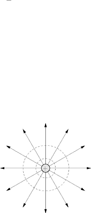
For a simple case of an isolated positive charge, the electric field is directed radially outward, as
shown in the Fig. 3.1, since a positively charged test particle would be repelled radially.

Electric Field and Equipotential: 2
Figure 3.1: Lines of force ( Solid Lines Radially Outward) and Equipotentials (Dashed Lines
Concentric Circles)
For the case of an isolated negative charge, the force lines are radially directed inward, as a
positively charged test particle would be attracted radially. The force lines are crowded together
where the field is stronger and are further apart where the field is weaker. The field has a (1/r
2
)
behavior; that is, it decreases inversely as the square of the distance from the isolated charge.
Experimentally we cannot truly map the field because of difficulties in placing the test charge at
a point in space and determining the force acting on the test charge. However, it is possible to
map the electric field indirectly from the equipotential lines. (In three dimensions, electric field is
mapped from equipotential surfaces.)
The potential difference ∆V between two points is defined as the work required to move a unit
positive charge from one point to the other in the electric field:
0
q
W
ΔV =
(2)
If the test charge q
0
is moved perpendicular to the electric field or the force lines, no work is
done or W = 0. This implies that ∆V = 0; that is, the potential remains constant along a path that
is perpendicular to the force lines. Such a path that has the same value of potential at all points
on it is called an equipotential line in two dimensions, and an equipotential surface in three
dimensions.
It can be easily shown that the electric field is given by the negative gradient of the potential. The
magnitude of the field is
ds
dV
ΔE =
(3)
where s is a coordinate in the direction of the electric field.
Two equipotential lines or two force lines from a given charge distribution never cross each
other, since both the potential and the electric field at any point other than the point-like charges
themselves always have unique values. At the location of a point-like charge, the equipotential
lines collapse to that point, and the lines of force diverge from a positive point-like charge and
converge into a negative point-like charge; see Fig. 3.1.

Electric Field and Equipotential: 3
PROCEDURE:
Figure 3.2: Experimental Setup.
1. Place the opaque template (for example, parallel-plate capacitor shown in the figure as
dark region) at the bottom of the field mapping board.
2. Fasten a piece of graph paper on the upper side of the mapping board by pressing on the
springs (located at the four corners) and push paper under the rubber stops and release the
springs.
3. Place the transparent/cardboard template on the graph sheet and align according to the
tiny holes located at the top of the template.
4. Turn the board upside down to ensure that the opaque template and the
transparent/cardboard template on the opposite side of the board are both aligned.
5. Carefully, slide the U-shaped probe into the board, with the ball end facing the underside
of the board.
6. Connect the potential source to the conducting terminals X and Y and make the
connections for the digital volt meter (DVM) with the terminal B as shown in the Fig.
3.2.
7. Turn on the potential source. Move the probe over the graph sheet to find a zero reading
position. This point must be at the same potential as B. Move the probe to another null
point and continue this procedure to find a series of these points.
8. Connect these equipotential points with a smooth curve to display the equipotential line
as B.
9. Move the digital voltmeter (DVM) connection to C now, and find the corresponding
equipotential line. (The DVM should indicate zero voltage).
10. Make a mark to identify this location.
11. Repeat the above procedure for all terminals (E1, E2, E3, etc) of the series of resistors.
12. Draw in, using dashed lines, the lines of force which are everywhere perpendicular to the
equipotential lines.
13. Repeat the experiment for the second template.
