
U.S. Department of the Interior
U.S. Geological Survey
Scientific Investigations Report 2020–5065
Prepared in cooperation with the U.S. Nuclear Regulatory Commission
Flood-Frequency Estimation for Very Low Annual
Exceedance Probabilities Using Historical, Paleoflood, and
Regional Information with Consideration of Nonstationarity
EXPLANATION
Mann-Kendall trend line for
systematic record and
historical peaks, p-value=0.01
Mann-Kendall trend line for
systematic record, p-value=0.33
●
1880 1900 1920 1940 1960 1980 2000 2020
Annual peak streamflow, in cubic feet per second
10
100
1,000
10,000
100,000
●
●
●
●
●
●
●
●
●
●
●
●
●
●
●
●
●
●
●
●
●
●
●
●
●
●
●
●
●
●
●
●
●
●
●
●
●
●
●
●
●
●
●
●
●
●
●
●
●
●
●
●
●
●
●
●
●
●
●
●
●
●
●
●
●
●
●
●
●
●
●
●
●
●
●
●
●
●
●
●
●
Trend lines
Lower reach, Rapid Creek, South Dakota
Annual peak streamflow
Historical peak
EXPLANATION
Observation (all peaks treated as consecutive)
Annual peak streamflow, in cubic feet per second
0 20 40 60 80 100
10
100
1,000
10,000
100,000
●
●
●
●
●
●
●
●
●
●
●
●
●
●
●
●
●
●
●
●
●
●
●
●
●
●
●
●
●
●
●
●
●
●
●
●
●
●
●
●
●
●
●
●
●
●
●
●
●
●
●
●
●
●
●
●
●
●
●
●
●
●
●
●
●
●
●
●
●
●
●
●
●
●
●
●
●
●
●
●
●
●
Lower reach, Rapid Creek, South Dakota
Mean of distribution of
annual peak streamflow
Annual peak streamflow
EXPLANATION
0.00010.010.1
1520
40
70
909899.5
Annual exceedance probability, in percent
10
100
1,000
10,000
100,000
1,000,000
10,000,000
100,000,000
Annual peak streamflow, in cubic feet per second
Peak fq v 7.2 run 10 /5/ 2019 1:53 :13 PM
Expected Moments Algorithm (E MA ) using
Weighted Skew option
0.407 = Skew (G)
Multiple Grubbs-Beck
0 Zeroes not displayed
0 Censored flows below PILF (LO) T hreshold
0 Gaged peaks below PILF (LO) Threshold
Fitted frequency
Confidence limit—5-percent lower,
95-percent upper
Censored flow
Interval flood estimate
Gaged peak
Historical peak
Lower reach, Rapid Creek, South Dakota
Cover. Upper left to bottom right, figures 21, 22, and 24.
Flood-Frequency Estimation for Very Low
Annual Exceedance Probabilities Using
Historical, Paleoflood, and Regional
Information with Consideration of
Nonstationarity
By Karen R. Ryberg, Kelsey A. Kolars, Julie E. Kiang, and Meredith L. Carr
Prepared in cooperation with the U.S. Nuclear Regulatory Commission
Scientific Investigations Report 2020–5065
U.S. Department of the Interior
U.S. Geological Survey
U.S. Department of the Interior
DAVID BERNHARDT, Secretary
U.S. Geological Survey
James F. Reilly II, Director
U.S. Geological Survey, Reston, Virginia: 2020
For more information on the USGS—the Federal source for science about the Earth, its natural and living resources,
natural hazards, and the environment—visit https://www.usgs.gov or call 1–888–ASK–USGS.
For an overview of USGS information products, including maps, imagery, and publications, visit
https://store.usgs.gov/.
Any use of trade, firm, or product names is for descriptive purposes only and does not imply endorsement by the U.S.
Government.
Although this information product, for the most part, is in the public domain, it also may contain copyrighted materials
as noted in the text. Permission to reproduce copyrighted items must be secured from the copyright owner.
Suggested citation:
Ryberg, K.R., Kolars, K.A., Kiang, J.E., and Carr, M.L., 2020, Flood-frequency estimation for very low annual
exceedance probabilities using historical, paleoflood, and regional information with consideration of nonstationarity:
U.S. Geological Survey Scientific Investigations Report 2020–5065, 89 p., https://doi.org/ 10.3133/ sir20205065.
Associated data for this publication:
U.S. Geological Survey, 2017, USGS water data for the Nation: U.S. Geological Survey National Water Information
System database, https://doi.org/10.5066/F7P55KJN.
ISSN 2328-0328 (online)
iii
Author Roles and Acknowledgments
Robert R. Mason, Jr. and Timothy A. Cohn of the U.S. Geological Survey (USGS) and Joseph
Kanney of the U.S. Nuclear Regulatory Commission (NRC) developed the project scope. The NRC
also developed the Statement of Work and actively participated in the design of the study. Karen
R. Ryberg (USGS) provided most of the draft text, including contributions to the literature review
section, and completed the initial data analysis and flood-frequency analyses. Kelsey A. Kolars
(USGS) completed most of the literature review on flood-frequency estimation in consideration
of stationary and nonstationary systems. Julie E. Kiang (USGS) contributed to the introduc-
tion, report structure, and revisions. Harry Jenter assisted with project scoping and oversight.
Ryberg, Kolars, Kiang, and Meredith L. Carr (NRC) compiled the report; all authors contributed to
addressing review comments. Steven K. Sando (USGS) and William H. Asquith (USGS) provided
technical reviews of all material, and Tara Williams-Sether (USGS) provided an additional
technical review of methods for including regional information. The NRC also contributed
technical comments. This work was funded by the U.S. Nuclear Regulatory Commission (NRC–
HQ–60–15–I–0006) with Carr acting as the Commission project manager.
The authors acknowledge the USGS Water Mission Area Nonstationarity Workgroup (of which
the USGS authors are members) for their in compiling a database of citations related to floods
under nonstationary conditions before the start of this project. Many of those citations were
used for this report.
v
Contents
Author Roles and Acknowledgments ........................................................................................................iii
Abstract ...........................................................................................................................................................1
Introduction.....................................................................................................................................................2
Purpose and Scope ..............................................................................................................................3
Limitations of Analysis .........................................................................................................................3
Literature Review of Stationary and Nonstationary Flood-Frequency Analysis .................................3
Flood-Frequency Analysis Background ............................................................................................3
Nonstationarity Detection ...................................................................................................................4
Analysis Tools ...............................................................................................................................5
U.S. Army Corps of Engineers Nonstationarity Detection Tool ...................................5
The TREND Tool ...................................................................................................................5
R Packages for Nonstationary Detection .......................................................................6
Factors that Contribute to Nonstationarity ..............................................................................7
Regulation ............................................................................................................................7
Land-Use Change ...............................................................................................................8
Climate Variability and Change .........................................................................................8
Long-Term Climate and Land Changes ............................................................................9
Including External Information ..................................................................................................9
Historical and Paleoflood Data .........................................................................................9
Historical Data ..........................................................................................................10
Paleoflood Data ........................................................................................................10
Use of Thresholds in Historical and Paleoflood Data ........................................11
Regional Data ....................................................................................................................12
Regional and Weighted Skew ................................................................................12
Regression Methods ...............................................................................................13
Regional Transfer .....................................................................................................13
Index Flood ................................................................................................................13
Region-of-Influence Approach ..............................................................................14
Methods and Tools for Examining Peak-Flow Series Characteristics and Associated
Statistical Assumptions .................................................................................................................14
Nonstationary Detection Methods ..................................................................................................15
Regional Analysis Tools .....................................................................................................................18
Sites Selected for Case Studies ................................................................................................................18
Red River of the North at Winnipeg, Manitoba, Canada ..............................................................20
Lower reach, Rapid Creek, South Dakota .......................................................................................20
Spring Creek, South Dakota ..............................................................................................................21
Cherry Creek near Melvin, Colorado ...............................................................................................21
Escalante River near Escalante, Utah .............................................................................................21
Data and Methods Used for Case Studies ..............................................................................................21
Data .......................................................................................................................................................22
Initial Data Analysis ............................................................................................................................22
Autocorrelation ..........................................................................................................................22
Change-Point Analysis ..............................................................................................................22
Monotonic Trend Analysis ........................................................................................................23
vi
Flood-Frequency Analysis ..........................................................................................................................23
Statistical Distribution Used .............................................................................................................24
Method for Estimating Distribution Parameters ............................................................................24
Potentially Influential Low Floods ....................................................................................................24
Case Study Results and Discussion .........................................................................................................24
Red River of the North at Winnipeg, Manitoba, Canada ..............................................................25
Autocorrelation ..........................................................................................................................26
Change-Point Analysis ..............................................................................................................26
Trend Analysis ............................................................................................................................27
Flood-Frequency Analysis ........................................................................................................27
Comparisons to Other Flood-Frequency Methods ......................................................32
Summary......................................................................................................................................36
Lower reach, Rapid Creek, South Dakota .......................................................................................40
Initial Data Analysis ...................................................................................................................40
Flood-Frequency Analysis ........................................................................................................40
Comparisons to Other Flood-Frequency Methods ......................................................42
Summary......................................................................................................................................42
Spring Creek, South Dakota ..............................................................................................................46
Initial Data Analysis ...................................................................................................................46
Flood-Frequency Analysis ........................................................................................................46
Comparisons to Other Flood-Frequency Methods ......................................................50
Summary......................................................................................................................................52
Cherry Creek near Melvin, Colorado ...............................................................................................54
Initial Data Analysis ...................................................................................................................54
Flood-Frequency Analysis ........................................................................................................54
Comparisons to Other Flood-Frequency Methods ......................................................56
Summary......................................................................................................................................58
Escalante River near Escalante, Utah .............................................................................................63
Initial Data Analysis ...................................................................................................................63
Flood-Frequency Analysis ........................................................................................................63
Comparisons to Other Flood-Frequency Methods ......................................................68
Summary......................................................................................................................................72
Summary........................................................................................................................................................74
References Cited..........................................................................................................................................76
Appendix 1. Data, Settings, and Output for Each Site and Scenario .................................................89
Figures
1. Map showing sites selected for detailed analysis of the peak-flow record and
for flood-frequency analysis .....................................................................................................19
2. Graph showing systematic, historical, and paleoflood peaks and historical
intervals for streamgage station 05OJ015 ..............................................................................25
3. Graph showing the autocorrelation for peaks in the systematic period of record
for streamgage station 05OJ015 ...............................................................................................26
vii
4. Graph showing change point in mean and variance for peaks in the systematic
period of record for streamgage station 05OJ015 .................................................................27
5. Graph showing Mann-Kendall test for trend in the annual peak-streamflow
record for streamgage station 05OJ015 ..................................................................................28
6. Graph showing peaks and thresholds used as input for flood-frequency
analysis scenarios 1 and 2 for streamgage station 05OJ015 ..............................................30
7. Graph showing annual exceedance probability plot and fitted distribution for
streamgage station 05OJ015 .....................................................................................................30
8. Graph showing systematic and historical peaks, paleo-derived peaks, and
historical and paleo-derived thresholds used for flood-frequency analysis
scenarios 9 and 10 for streamgage station 05OJ015 ............................................................31
9. Graph showing annual exceedance probabilities for streamgage station
05OJ015 with the input data depicted in figure 8 and at-site skew (scenario 9) .............31
10. Graph showing annual exceedance probabilities for streamgage station
05OJ015 with the input data depicted in figure 8 and weighted skew (scenario 10) ......32
11. Graph showing point and interval estimates for streamgage station 05OJ015
floods with annual exceedance probability of 0.10, calculated using U.S.
Geological Survey PeakFQ software version 7.2 under 10 different scenarios ...............33
12. Graph showing point and interval estimates for streamgage station 05OJ015
floods with annual exceedance probability of 0.01, calculated using U.S.
Geological Survey PeakFQ software version 7.2 under 10 different scenarios
and 13 additional point estimates from other flood-frequency studies .............................33
13. Graph showing point and interval estimates for streamgage station 05OJ015
floods with annual exceedance probability of 1×10
−3
, calculated using U.S.
Geological Survey PeakFQ software version 7.2 under 10 different scenarios ...............34
14. Graph showing point and interval estimates for streamgage station 05OJ015
floods with annual exceedance probability of 1×10
−4
..........................................................34
15. Graph showing point and interval estimates for streamgage station 05OJ015
floods with annual exceedance probability of 1×10
−5
..........................................................35
16. Graph showing point and interval estimates for streamgage station 05OJ015
floods with annual exceedance probability of 1×10
−6
..........................................................35
17. Graphs showing point and interval estimates for a range of annual exceedance
probabilities for streamgage station 05OJ015 floods, calculated using U.S.
Geological Survey PeakFQ software version 7.2, with at-site and weighted
skew and the systematic record only .....................................................................................38
18. Graphs showing point and interval estimates for a range of annual exceedance
probabilities for streamgage station 05OJ015 floods, calculated using U.S.
Geological Survey PeakFQ software version 7.2 with at-site and weighted
skew and the systematic record plus historical peaks and thresholds and
paleo-derived peaks and paleo-derived thresholds .............................................................39
19. Graph showing systematic peaks and historical peaks for lower reach, Rapid
Creek, South Dakota ...................................................................................................................40
20. Graph showing the autocorrelation for peaks in systematic period of record for
lower reach, Rapid Creek, South Dakota ................................................................................41
21. Graph showing change points in mean and variance for peaks in systematic
period of record for lower reach, Rapid Creek, South Dakota ............................................41
22. Graph showing Mann-Kendall test for trend in the peak-streamflow record for
lower reach, Rapid Creek, South Dakota ................................................................................42
viii
23. Graph showing systematic and historical peaks, paleo-derived interval peaks,
and historical and paleo-derived thresholds used as input for flood-frequency
analysis with weighted skew, lower reach, Rapid Creek, South Dakota ..........................43
24. Graph showing annual exceedance probability plot and fitted distribution for
lower reach of Rapid Creek, South Dakota, using the input data depicted in
figure 23 and weighted skew ....................................................................................................43
25. Graph showing point estimates and confidence bounds for scenarios using U.S.
Geological Survey PeakFQ software version 7.2 for lower reach of Rapid Creek,
South Dakota, for floods with annual exceedance probability of 0.01 ..............................44
26. Graphs showing point and interval estimates for a range of annual exceedance
probabilities for lower reach of Rapid Creek, South Dakota, floods, calculated
using U.S. Geological Survey PeakFQ software version 7.2 with weighted skew
and systematic data and with systematic plus historical data ...........................................45
27. Graph showing point and interval estimates for a range of annual exceedance
probabilities for lower reach of Rapid Creek, South Dakota, floods, calculated
using U.S. Geological Survey PeakFQ software version 7.2, with weighted skew
and systematic, historical, and paleoflood data ....................................................................46
28. Graph showing the autocorrelation for peaks in systematic period of record for
Spring Creek, South Dakota ......................................................................................................47
29. Graph showing change points in mean and variance for peaks in systematic
period of record for Spring Creek, South Dakota ..................................................................47
30. Graph showing Mann Kendall test for trend in the peak-streamflow record for
Spring Creek, South Dakota ......................................................................................................48
31. Graph showing systematic and paleo-derived interval peaks and thresholds
used as input for flood-frequency analysis with weighted skew, Spring Creek,
South Dakota ...............................................................................................................................49
32. Graph showing annual exceedance probability plot and fitted distribution for
Spring Creek, South Dakota ......................................................................................................49
33. Graph showing interval peaks predicted from lower reach Rapid Creek,
thresholds, and systematic data ..............................................................................................50
34. Graph showing annual exceedance probability plot and fitted distribution for
Spring Creek, South Dakota ......................................................................................................51
35. Graph showing point estimates and confidence bounds for PeakFQ scenarios
for Spring Creek, South Dakota, for floods with annual exceedance
probability of 0.01 ........................................................................................................................51
36. Graphs showing point and interval estimates for a range of annual exceedance
probabilities for Spring Creek, South Dakota, floods, calculated using U.S.
Geological Survey PeakFQ software version 7.2, with weighted skew and
systematic data and with systematic plus paleoflood data ................................................53
37. Graph showing point and interval estimates for a range of annual exceedance
probabilities for Spring Creek, South Dakota, floods, calculated using U.S.
Geological Survey PeakFQ software version 7.2, with weighted skew and
systematic, historical, and predicted paleoflood data .........................................................54
38. Graph showing the autocorrelation for peaks in systematic period of record for
streamgage station 06712500 ....................................................................................................55
39. Graph showing change points in mean and variance for peaks in systematic
period of record for streamgage station 06712500 ................................................................55
40. Graph showing Mann-Kendall test for trend in the peak-streamflow record for
streamgage station 06712500 ....................................................................................................56
ix
41. Graph showing annual exceedance probability plot and fitted distribution for
streamgage station 06712500 using systematic data only and weighted skew ...............57
42. Graph showing annual exceedance probability plot and fitted distribution
for streamgage station 06712500 using systematic and paleoflood data with
weighted skew ............................................................................................................................57
43. Graph showing point estimates for streamgage station 06712500 flood with
annual exceedance probability of 0.10 ...................................................................................58
44. Graph showing point estimates for streamgage station 06712500 flood with
annual exceedance probability of 0.01 ...................................................................................59
45. Graphs showing point estimates for streamgage station 06712500 flood with
annual exceedance probability of 1×10
−3
...............................................................................59
46. Graph showing point estimates for streamgage station 06712500 flood with
annual exceedance probability of 1×10
−4
...............................................................................60
47. Graph showing point estimates for streamgage station 06712500 flood with
annual exceedance probability of 1×10
−5
...............................................................................60
48. Graph showing point estimates for streamflow-gaging station 06712500 flood
with annual exceedance probability of 1×10
−6
......................................................................61
49. Graphs showing point and interval estimates for a range of annual exceedance
probabilities for streamgage station, calculated using U.S. Geological Survey
PeakFQ software version 7.2, with weighted skew and no paleoflood data and
with weighted skew and systematic and paleoflood data ..................................................62
50. Graph showing the autocorrelation for peaks in systematic period of record for
streamgage station 09337500, 1943–55 ...................................................................................64
51. Graph showing the autocorrelation for peaks in systematic period of record for
streamgage station 09337500, 1972–2015 ...............................................................................64
52. Graph showing change points in mean and variance for peaks in systematic
period of record for streamgage station 09337500, 1943–55 ...............................................65
53. Graph showing change points in mean and variance for peaks in systematic
period of record for streamgage station 09337500, 1972–2015 ...........................................65
54. Graph showing Mann Kendall test for trend in the peak-streamflow record for
streamgage station 09337500 ....................................................................................................66
55. Graph showing peaks and thresholds for flood-frequency analysis,
streamgage station 09337500 ....................................................................................................66
56. Graph showing annual exceedance probabilities for streamgage station
09337500 using the systematic peaks only .............................................................................67
57. Graph showing annual exceedance probabilities for streamgage station
09337500 using the input data depicted in figure 55 .............................................................67
58. Graph showing annual exceedance probabilities for streamgage station
09337500 using systematic, historical, and paleoflood peaks and thresholds .................68
59. Graph showing point estimates and confidence bounds for streamgage station
09337500 floods with annual exceedance probability of 0.10, calculated under
three different scenarios using U.S. Geological Survey PeakFQ software
version 7.2 ....................................................................................................................................69
60. Graph showing point estimates and confidence bounds for streamgage station
09337500 floods with annual exceedance probability of 0.01, calculated under
three different scenarios using U.S. Geological Survey PeakFQ software
version 7.2 compared to five point estimates from other studies .......................................69
61. Graph showing point estimates and confidence bounds for streamgage station
09337500 floods with annual exceedance probability of 1×10
−3
.........................................70
x
62. Graph showing point estimates and confidence bounds for streamgage station
09337500 floods with annual exceedance probability of 1×10
−4
.........................................70
63. Graph showing point estimates and confidence bounds for streamgage station
09337500 floods with annual exceedance probability of 1×10
−5
.........................................71
64. Graph showing point estimates and confidence bounds for streamgage station
09337500 floods with annual exceedance probability of 1×10
−6
.........................................71
65. Graphs showing point and interval estimates for a range of annual exceedance
probabilities for streamgage station 09337500 floods, calculated using U.S.
Geological Survey PeakFQ version 7.2, with weighted skew and systematic
data and with weighted skew systematic plus historical data ...........................................73
66. Graph showing point and interval estimates for a range of annual exceedance
probabilities for streamgage station 09337500 floods, calculated using U.S.
Geological Survey PeakFQ version 7.2, with weighted skew and systematic,
historical, and paleoflood data .................................................................................................74
Tables
1. Parametric and nonparametric approaches for detection of abrupt and gradual
nonstationarity ............................................................................................................................16
2. Sites selected for flood-frequency analysis ..........................................................................20
3. Trend results for streamgage station 05OJ015, 1907–2016, using modifications
of the Mann-Kendall test for trend ..........................................................................................29
4. Streamflow estimates for selected annual exceedance probabilities and
associated confidence intervals (lower and upper) and variance estimates for
flood-frequency analysis under 10 different scenarios using U.S. Geological
Survey PeakFQ software (Veilleux and others, 2014) version 7.2 for streamgage
station 05OJ015 as well as results from flood-frequency studies by Burn and
Goel (2001) and Harden (1999) ..................................................................................................29
5. Streamflow estimates for selected annual exceedance probabilities and
associated confidence intervals (lower and upper) and variance estimates for
flood-frequency analysis under three different scenarios using U.S. Geological
Survey PeakFQ software version 7.2 for the lower reach of Rapid Creek, South
Dakota, with comparisons to Harden and others (2011) ......................................................40
6. Streamflow estimates for selected annual exceedance probabilities and
associated confidence intervals (lower and upper) and variance estimates for
flood-frequency analysis under three different scenarios using U.S. Geological
Survey PeakFQ software version 7.2 for Spring Creek, South Dakota, with
comparisons to Harden and others (2011) ..............................................................................46
7. Streamflow estimates for selected annual exceedance probabilities and
associated confidence intervals (lower and upper) and variance estimates for
flood-frequency analysis under two different scenarios using U.S. Geological
Survey PeakFQ software version 7.2 for streamgage station 06712500 with
comparisons to other distributions and fitting methods ......................................................56
8. Streamflow estimates for selected annual exceedance probabilities and
associated confidence intervals (lower and upper) and variance estimates for
flood-frequency analysis under three different scenarios using U.S. Geological
Survey PeakFQ software version 7.2 for streamgage station 09337500 with
comparisons to Webb and others (1988), Webb and Rathburn (1988), and
Kenney and others (2008) ..........................................................................................................63

xi
Conversion Factors
U.S. customary units to International System of Units
Multiply By To obtain
Length
foot (ft) 0.3048 meter (m)
mile (mi) 1.609 kilometer (km)
Area
square mile (mi
2
) 2.590 square kilometer (km
2
)
Volume
acre-foot (acre-ft) 1,233 cubic meter (m
3
)
Flow rate
cubic foot per second (ft
3
/s) 0.02832 cubic meter per second (m
3
/s)
International System of Units to U.S. customary units
Multiply By To obtain
Length
meter (m) 3.281 foot (ft)
kilometer (km) 0.6214 mile (mi)
Area
square kilometer (km
2
) 0.3861 square mile (mi
2
)
Volume
cubic meter (m
3
) 35.31 cubic foot (ft
3
)
Flow rate
cubic meter per second (m
3
/s) 35.31 cubic foot per second (ft
3
/s)
xii
Abbreviations
acf autocorrelation function
AEP annual exceedance probability
EMA Expected Moments Algorithm
H Hurst exponent coefficient
LTP long-term persistence
Ma megaanum or million years
MBIC modified Bayes information criterion
MKT Mann-Kendall test for monotonic trend
MLE maximum likelihood estimation
MOVE maintenance of variance extension
MOVE.3 Maintenance of Variance Extension Type III
NRC U.S. Nuclear Regulatory Commission
PE3 Pearson type III distribution (three-parameter probability distribution)
PFF peak-flow file
PILF potentially influential low flood
PMF probable maximum flood
PREC probabilistic regional envelope curve
Q streamflow
ROI region of influence
STP short-term persistence
USACE U.S. Army Corps of Engineers
USGS U.S. Geological Survey

Flood-Frequency Estimation for Very Low Annual
Exceedance Probabilities Using Historical, Paleoflood,
and Regional Information with Consideration of
Nonstationarity
By Karen R. Ryberg,
1
Kelsey A. Kolars,
1
Julie E. Kiang,
1
and Meredith L. Carr
2
Abstract
Streamow estimates for oods with an annual exceed-
ance probability of 0.001 or lower are needed to accurately
portray risks to critical infrastructure, such as nuclear power-
plants and large dams. However, extrapolating ood-frequency
curves developed from at-site systematic streamow records
to very low annual exceedance probabilities (less than 0.001)
results in large uncertainties in the streamow estimates.
Traditionally, methods for statistically estimating ood fre-
quency have relied on the systematic streamow record, which
provides a time series of annual maximum ood peaks, often
including some historical peaks. However, most peak-ow
records are less than 100 years, and uncertainties are large
when trying to extrapolate magnitudes of very low annual
exceedance probability events.
Other data may be available that extend the record
beyond the systematic dataset. Historical data are dened as
data from outside the period of systematic records but within
the period of human records. Examples of historical informa-
tion include ood estimates from other agencies and newspa-
per accounts that can be translated to ood magnitude point
estimates, interval estimates, or perception thresholds (such
as a statement that an 1880 ood was the largest since 1869).
Paleoood data, which may also extend the dataset, include a
broad range of information about ood occurrence or magni-
tude from sources like sediment deposits or tree rings.
Several assumptions are made in ood-frequency analy-
sis, and an understanding of whether the data conform to
these assumptions is desired. A particularly dicult assump-
tion to evaluate for ood-frequency analysis is the underlying
assumption that the ood series is stationary—the assumption
that a time series of peak ow varies around a constant mean
within a particular range of values (constant variance). As the
hydrologic community’s understanding of natural systems
and anthropogenic eects on streamows has evolved, the
1
U.S. Geological Survey.
2
U.S. Nuclear Regulatory Commission.
community has come to understand that many surface-water
systems exhibit one or more forms of nonstationarity, and thus
the stationarity assumption is often violated to some degree.
However, there is currently (2020) no consensus among
hydrologists regarding the most appropriate ood-frequency-
analysis methods for nonstationary systems, and this topic
remains an active area of research.
A literature review was completed to summarize the state
of the science of ood frequency. The literature review high-
lights tools available to detect nonstationarities and identies
approaches that include external information to inform ood-
frequency analysis. To demonstrate methods for initial data
analysis and for incorporating historical and paleoood infor-
mation in ood-frequency analysis, ve sites were selected:
the Red River of the North at James Avenue Pumping Station,
Winnipeg, Manitoba, Canada; lower reach, Rapid Creek,
South Dakota; Spring Creek, South Dakota; Cherry Creek near
Melvin, Colorado; and Escalante River near Escalante, Utah.
The sites were chosen for the availability of published histori-
cal and paleoood data and for their geographic diversity
and unique characteristics, which highlighted issues such as
autocorrelation, change points, trends, outlier peaks, or short
periods of record.
An initial data analysis that involved examining records
for autocorrelation, change points, and trends was completed
for all sites. The ood-frequency analysis completed for this
study used version 7.2 of the U.S. Geological Survey PeakFQ
program. Multiple analyses were done on each site document-
ing the change in the ood-frequency curve when additional
historical or paleoood data were added. When other ood-
frequency studies were available, their results were compared
to the results here. The comparisons in some cases simply
show the eect of additional years of data, whereas other com-
parisons show results from probability distributions or tting
methods other than those used in PeakFQ.
For the Red River of the North, ood-frequency analy-
sis shows that paleoood data appear necessary to reason-
ably estimate very low annual exceedance probabilities. For
the analysis of the lower reach of Rapid Creek and Spring
Creek, paleoood information helped put a high outlier from
2 Flood-Frequency Estimation for Very Low Annual Exceedance Probabilities
the systematic period in context; however, very low annual
exceedance probabilities at these sites still had extraordi-
narily large condence bounds. These sites also showed that
paleoood information might be transferred from one site
to another, with the caveat that this is a case where we had
existing paleoood data to test the transfer of paleoood
information—this is not the case at many sites, and transfer-
ring paleoood information requires assumptions about the
comparability of oods at the sites. The Cherry Creek analysis
armed the result of an earlier study that showed that the
generalized Pareto distribution was not a good distribution
for estimating very low annual exceedance probabilities. The
Escalante River analysis showed that adding paleoood infor-
mation might increase uncertainty for very low annual exceed-
ance probabilities, compared to analysis with the systematic
period of record information only, when the paleoood peaks
are of much larger magnitudes than the systematic record.
Introduction
The U.S. Geological Survey (USGS), with cooperation
and funding from the U.S. Nuclear Regulatory Commission
(NRC), has investigated the application of statistical analysis
methods and tools for probabilistic ood hazard assessment,
focusing on low probability oods. Estimating the frequency
and magnitude of low probability oods is needed to quantify
ood risks for critical infrastructure, such as nuclear power-
plants and large dams. These oods are dened as events hav-
ing “very low” annual exceedance probabilities (AEPs), less
than 0.001 (as in Asquith and others, 2017); scientic nota-
tion is used to represent these very low AEPs, such as 1×10
−3
for 0.001. Although oods with an AEP of 1×10
−4
might be
considered exceptionally rare from a hydrological perspec-
tive, they are not exceptionally rare from a nuclear powerplant
safety perspective. In fact, nuclear powerplant design-basis
events hazards (for example, large break loss of coolant acci-
dents) often have a frequency in the range of 1×10
−5
per year
and lower (Tregoning and others, 2008).
Standard ood-frequency analysis approaches rely on
a time series of annual maximum streamow (hereinafter
referred to as “peak ow”), derived from the at-site system-
atic record. The time series is t to a statistical distribution
to estimate ood quantiles, and the analysis requires several
assumptions about the data. A concern for ood-frequency
analysis is the underlying assumption that the peak-ow series
is stationary. A stationary peak-ow series has been recorded
within a consistent (albeit potentially highly variable) hydro-
climatic system with long-term consistency in the fundamental
ood-generating processes. Statistically, a stationary peak-
ow series varies around a constant mean within a particular
range of values according to a dened variance (spread of the
distribution). As the hydrologic community’s understanding
of natural systems and anthropogenic eects on streamows
has evolved, the community has come to understand that many
surface-water systems exhibit one or more forms of nonsta-
tionarity, and thus the stationarity assumption is often violated
to some degree. Nonstationarity is a statistical property of a
peak-ow series such that the long-term distributional proper-
ties (the mean, variance, or skew) change one or more times
either gradually or abruptly through time. Individual nonsta-
tionarities may be attributed to one source (for example, either
regulation, land-use change, or climate) but often are the result
of a mixture of those sources (Vogel and others, 2011), mak-
ing detection and attribution of nonstationarities challenging.
However, detection and attribution can inform ood-frequency
analysis. Currently, there is no consensus among hydrologists
regarding the most appropriate frequency-analysis methods to
use for nonstationary systems, and this topic remains an active
area of research.
An additional concern in tting the ood-frequency
curve is the availability of data. The systematic streamow
records that form the basis of the analysis are typically short
(the oldest USGS streamow records start in the late 1800s,
and records exceeding 100 years in length are scarce), and
large uncertainties remain when trying to extrapolate to very
low AEPs.
Other data may be available that extend the period of
record beyond the systematic dataset. Historical data are
dened as data from outside the period of systematic records,
yet within the period of human records, such as newspaper
accounts that can be used to calculate to ood magnitude point
estimates, interval estimates, or perception thresholds (such as
a statement that an 1880 ood was the largest since 1869).
Paleoood data, which may also extend the dataset,
include a broad range of information about ood occurrence or
magnitude from sources like sediment deposits or tree rings.
Paleoood data are generally not available in the USGS peak-
ow le (PFF) or the streamow databases of other agencies
but are published in paleoood studies.
The purpose of this work was to complete some of the
tasks in a work plan the NRC and USGS developed to inves-
tigate the state of practice for using and characterizing the
uncertainties of statistical analytical tools for assessing very
low AEPs (less than 0.001, that is oods that have an average
recurrence interval of less than 1,000 years, see Holmes and
Dinicola [2010] for more information). Asquith and others
(2017) completed the rst task of the plan, which was to better
understand the uncertainty of ood-frequency estimates when
they are determined from peaks collected as part of a regu-
lar program of streamow collection to produce systematic
records of peak ow. The later tasks, which are the focus of
this work, were to explore methods used to identify and char-
acterize nonstationarities and to investigate the possible usage
of additional sources of information (especially historical
and paleoood data and regionalization) that may extend the
record and aect the uncertainty of ood-frequency estimates
for very low AEPs.
The rst goal of this work is to explore how to identify if
a hydrologic system may be changing over time (nonstationar-
ity). Tools available to detect nonstationarities are discussed,
Literature Review of Stationary and Nonstationary Flood-Frequency Analysis 3
possible attributing factors are identied, and eorts to include
external information for detection of nonstationarities are
reviewed. Additionally, the work contributes to the under-
standing of underlying causes of nonstationarities and poten-
tial ways to address nonstationarities, while showing that the
problem is not easy to address.
The second goal of this work is to describe and demon-
strate how information about peak ows outside the system-
atic record can be incorporated into statistical ood-frequency
analysis to improve ood-frequency estimates and accurately
characterize and quantify uncertainty through the incorpo-
ration of historical, paleoood, and regional information.
Historical, paleoood, and regional information are reviewed,
and methods and tools to incorporate this information into
ood-frequency analysis are described and tested.
Purpose and Scope
The purpose of this report is to describe methods for
ood-frequency estimation for very low AEPs using histori-
cal, paleoood, and regional information with consideration
of nonstationarity. This report has two main sections. The
rst section discusses methods to detect nonstationarities and
reviews some suggested methods for dealing with nonstation-
arities. The second section demonstrates the use of historical
and paleoood data and of regional information to extend or
inform the record. Together, this report and Asquith and others
(2017) are intended to serve as a resource for NRC technical
sta, collaborators, and other parties interested in studying the
exposure of critical infrastructure, such as nuclear powerplants
and large dams. Conventions established in Asquith and others
(2017) are continued in this report.
For this work, ve sites were selected to demonstrate
methods for initial data analysis and to incorporate histori-
cal, paleoood, and regional information into ood-frequency
analyses. The sites were chosen because published historical
or paleoood data were available for them and because of their
geographic diversity and unique characteristics, some of which
highlighted issues such as autocorrelation, change points,
trends, outlier peaks, or short periods of record.
Limitations of Analysis
This report describes methods and illustrates their use
through their application to selected sites. Some subjectivity is
inherent in assessing the validity of historical and paleoood
data and in incorporating thresholds for missing periods during
the systematic record and for paleo periods. Local or regional
experts might make dierent choices when assessing these
sites. In addition, ood-frequency analysis under nonstationary
conditions is an active area of research, and many suggested
methods are not yet able to be incorporated into currently
available software or cannot incorporate historical or paleo-
ood data. Therefore, the ood-frequency results reported
here should not be considered denitive for design purposes
at any of these sites. The ood-frequency results are described
as case studies to indicate that these studies are examples of
using state of practice techniques to assess nonstationarity and
to better characterize very low AEPs.
Literature Review of Stationary and
Nonstationary Flood-Frequency
Analysis
An important consideration for any ood-frequency
analysis is whether a hydrologic system meets the assump-
tion of stationarity underpinning ood-frequency analysis.
Stationarity is a statistical concept meaning the underlying
distribution of a process does not change when shifted in time.
In the context of streamow, stationarity means that ows
vary within a particular window of variability around a long-
term mean.
Milly and others (2008) concluded that the assump-
tion of stationarity in water resources is “dead” because of
anthropogenic changes to Earth’s climate and has long been
compromised because of anthropogenic disturbance to the
landscape. However, Villarini and others (2009, p. 1) stated
that it is “easier to proclaim the demise of stationarity of ood
peaks than to prove it through analyses of annual ood peak
data.” The stationarity issue is not limited to anthropogenic
change though. A system can exhibit long-term “excursions,”
such as a multidecadal drought that may be part of the sys-
tem’s natural variation about a mean, but that excursion may
be dicult to distinguish from an anthropogenic change that
altered the system (Cohn and Lins, 2005). Methods have been
developed to treat hydrologic time series with these excursions
as scaled stochastic processes (Hamed, 2008; Koutsoyiannis,
2003; Koutsoyiannis, 2006). In other cases, it has been shown
through tree-ring proxy records that some hydrologic regimes
have likely never been stationary and that many records of
hydrologic observation are too short to be representative of
the long-term properties of the systems (Razavi and others,
2015). Flood-frequency analysis of nonstationary peak ows
is an area of active research without a clear path forward if
one declares the stationarity assumption cannot be used. The
following literature review discusses tools available to detect
individual nonstationarities, identies possible attributing
factors, and reviews eorts to include external information
for detection of nonstationarities. The review contributes to
the understanding of underlying causes of nonstationarity and
potential ways to address nonstationarities, while showing that
the problem is not easy to address.
Flood-Frequency Analysis Background
Around the late 1800s, the United States began to
establish an extensive streamgaging network, today (2020)
known as the USGS Streamgaging Network, with the rst
4 Flood-Frequency Estimation for Very Low Annual Exceedance Probabilities
gaging station constructed in 1889 along the Rio Grande
(U.S. Geological Survey, 2014). As the accumulation of
streamow data grew, so did the need for a nationwide stan-
dard for analyzing the data and determining ood frequencies.
Fuller (1914) published the rst method to estimate ood
frequencies nationwide. It was an innovative approach in that
it used principles of probability; however, the method assumed
ood frequencies could be calculated from short peak-ow
records provided one had records from several streams
(Rumsey, 2015). Fuller’s work was improved upon by Hazen
(1930) with technical renements and a discussion of how
ood-frequency analysis could be applied to understanding the
risk associated with ood protection, such as levees (Rumsey,
2015). Initially, ood-frequency analysis was completed by
private entities, but the Government increasingly became
involved in ood protection and oodplain management and,
therefore, had a growing interest in ood frequency. The
USGS published a Water Supply Paper on ood magnitude
and frequency in 1936 (Jarvis, 1936). Over the next 30 years,
there was a growing interest in ood insurance and ood-loss
control (Rumsey, 2015). In a 1966 U.S. Government report by
the U.S. Task Force on Federal Flood Control Policy, President
Lyndon Johnson’s letter of transmittal to the U.S. House of
Representatives stated, “… a Great Society cannot rest on
the achievements of the past. It must constantly strive to
develop new means to meet the needs of the people… The
task force report lays stress on actions which can and should
be immediately undertaken—To improve basic knowledge
about the ood hazard…” (U.S. Task Force on Federal Control
Policy, 1966, p. III–IV). To improve ood hazard knowledge,
the report recommended specic actions, including that “a
uniform technique of determining ood frequency should
be developed by a panel of the Water Resources Council”
(U.S. Task Force on Federal Control Policy, 1966, p. 1). The
Water Resources Council Hydrology Committee’s work
resulted in a 1967 publication of a report titled “A Uniform
Technique for Determining Flood Frequencies,” known as
“Bulletin 15” (Water Resources Council, 1967). Since then,
this Bulletin has been revised several times (Bulletin 17, U.S.
Water Resources Council, 1977; Bulletin 17A, U.S. Water
Resources Council, 1976; Bulletin 17B, Interagency Advisory
Committee on Water Data, 1982; and Bulletin 17C, England
and others, 2019), and software has been developed to assist
with analysis (England and others, 2019; Flynn and others,
2006). In the most recent Bulletin (Bulletin 17C; England
and others, 2019), as with the previous bulletins, the ood-
frequency methods rely on the assumption that the data are
stationary, independent and identically distributed, and lack
any short- or long-term persistence (STP or LTP; serial or
autocorrelation of values in the time series with lags greater
than 1 year). For some basins, these assumptions hold true,
and the methods suggested in Bulletin 17C are sucient; for
others, the methods suggested in Bulletin 17C may result in
incorrect conclusions. As more information becomes avail-
able through historical and paleoood records, there have
been questions about whether the hydrologic system ever was
stationary and if some apparent nonstationarities are simply
the result of LTP or autocorrelation (Cohn and Lins, 2005).
Nonstationarity, as discussed in this report, refers to
peak-ow distributions with either gradual or abrupt changes
in mean, variance, or both. Individual nonstationarities may be
attributed to one source (for example, either regulation, land-
use change, or climate) but often are the result of a mixture
of those sources (Vogel and others, 2011), making detection
dicult.
The diculties associated with detection and attribution
of nonstationarities have prompted much research. Review
papers and workshop discussions are available and serve
as guides to help determine the best methods for detecting
nonstationarities and to oer suggestions on potential causes
for nonstationarities detected (Kundzewicz and Robson,
2000, 2004; Olsen and others, 2010; Working Group 4 Flood
Frequency Estimation Methods and Environmental Change,
2013). Software tools have been created that incorporate sev-
eral well-known tests used for determining abrupt or gradual
changes that make detecting nonstationarities quicker, easier,
and more consistent. These software tools are publicly avail-
able, such as the U.S. Army Corps of Engineers (USACE)
Nonstationarity Tool (Friedman and others, 2016; U.S. Army
Corps of Engineers, 2016), TREND software (Chiew and
Siriwardena, 2005), and change-point analysis add-on pack-
ages for the statistical analysis software R (R Core Team,
2019), such as changepoint (Killick and Eckley, 2014), ecp
(James and Matteson, 2014), and cpm (Ross, 2015). Other
resources, such as websites like The Changepoint Repository
(Killick and others, 2012b), have been created to aid analysts
in locating references to techniques and methods related to
nonstationarity. These are just some of the many resources
available to those inquiring about nonstationarities in their
streamow records and how to deal with them.
Nonstationarity Detection
Consideration of nonstationarity in ood-frequency
analysis starts with selecting an appropriate nonstationarity-
detection method and determining the cause of detected
nonstationarities. Selecting an appropriate detection method
involves a thorough understanding of the data being analyzed;
this understanding is gained by examining the data for auto-
correlation, LTP, seasonality, independence, or non-normalities
(such as skew; Kundzewicz and Robson, 2004). Method selec-
tion also requires a clear understanding of the type of nonsta-
tionarity of interest, whether looking for a nonstationarity in
the mean, median, variance, or other parameter dening the
peak-ow distribution, or attempting to locate a nonstationar-
ity in the form of a gradual trend. Specically, a detected non-
stationarity in the underlying distribution could be the result
of a change in the distributional parameters or of changing
Literature Review of Stationary and Nonstationary Flood-Frequency Analysis 5
from one distribution to another (Friedman and others, 2016).
Even with a variety of available detection methods, it can be
dicult to detect nonstationarity in peak-ow series.
Traditionally, nonstationarity-detection methods have
tested time series for trends, abrupt changes in the mean or
variance, or changes in frequency (He and others, 2013).
Tests for abrupt changes in higher-order statistics, or higher
moments, of statistical distributions (such as skew, the third
moment about the mean, or kurtosis, the fourth moment
about the mean) exist (He and others, 2013) but are less apt
to be examined because changes in the mean are sensitive to
changes in skew and skew and kurtosis are functions of both
mean and variance (Abramowitz and Stegun, 1965). Many
change-point methods that identify abrupt nonstationarities
search for a change in the mean (Friedman and others, 2016,
2018; Ryberg and others, 2020). These generally do not work
well for peak ow because of skew in the data, and change-
point tests for changes in the median can be more successful
(Ryberg and others, 2020).
The relation between streamow and certain climatic
factors (temperature and precipitation) can further complicate
analysis because nonstationarities detected in temperature
or precipitation may not be reected in the peak-ow series
(Hirsch, 2011). Extreme caution is advised when reporting on
or using detected nonstationarities without a clear understand-
ing of what caused the nonstationarity. Attributing a non-
stationarity to regulation or land-use changes may be easier
than climate and even easier than attributing it to a mixture of
regulation and land-use change with climate.
Autocorrelated (or serially correlated) peak-ow series
have persistence or memory in that each peak is not a random
process but is related to one or more of the previous peaks.
Change points, or step trends, are abrupt changes in distri-
butional parameters of a time series dened by a particular
statistical distribution or are abrupt changes in median or
scale in a series of unknown statistical distribution. Trends are
gradual increases (or decreases) in peak ow over time and
are a violation of the assumption of independent identically
distributed observations. Flood-frequency analysis is based on
the assumption of independent, identically distributed obser-
vations. Autocorrelated series, series with change points and
series with trends, violate this assumption and are therefore
nonstationarities.
Analysis Tools
Publicly available tools to assist with detecting non-
stationarities in time series datasets include the USACE
Nonstationarity Detection Tool (U.S. Army Corps of
Engineers, 2016), TREND software (Chiew and Siriwardena,
2005), and a series of R packages and functions. These tools
ensure methods for detecting nonstationarities remain consis-
tent at diering locations and with dierent datasets. Each tool
implements a variety of nonstationarity-detection methods to
aid the user, but each tool also requires that the data satisfy
certain assumptions. Findings of a statistical nonstationarity
should be supported by documented changes to the hydrologic
system such as regulation, land-use change, or signicant
climatic events.
U.S. Army Corps of Engineers Nonstationarity Detection
Tool
The USACE Nonstationarity Detection Tool is intended
to aid users in assessing the stationarity of streamow records
in support of planning and engineering decision mak-
ing (Friedman and others, 2016, 2018). The tool has been
designed to produce consistent results across dierent loca-
tions and to be more convenient to apply than the TREND
Tool or R packages (although the Nonstationarity Detection
Tool itself is based on underlying R packages). The USACE
Nonstationarity Detection Tool does not require the user to
input time-series data (the user selects from a preset menu
of individual USGS streamgages). Application of the tool is
restricted to streamgages with at least 30 years of peak-ow
records (the tool will automatically identify streamgages with
sucient record length). These features may make the tool
convenient for novice users but also make the tool restrictive
to specied USGS streamgage locations. The tool implements
12 statistical methods for nonstationarity detection that include
parametric (based on estimates of distributions parameters)
and nonparametric (making no assumptions about a particular
distribution) approaches, gradual changes or abrupt change
points, single/multiple change points, change points in the
mean/variance/distribution, and a test for serial correlation
that, depending on the result, further limits the options avail-
able (Friedman and others, 2016). The restrictions associated
with the USACE Nonstationarity Detection Tool enforce
consistent nonstationarity detection at dierent locations and
support acceptance of the tool as meeting the guidelines for
certain Federal agencies (Friedman and others, 2016).
The TREND Tool
The TREND Tool was developed in Australia for use
by hydrologists, scientists, and consultants to aid in detect-
ing trends, change points, and randomness in the data. The
TREND Tool not only detects trends, as the name implies,
but also detects abrupt changes in annual streamow and
precipitation and includes a test for serial correlation. The
TREND Tool implements methods from Grayson and others
(1996) and Kundzewicz and Robson (2000). Like the USACE
Nonstationarity Detection Tool, the TREND Tool provides
methods for detecting nonstationarities. The TREND Tool can
be considered more exible than the USACE Nonstationarity
Detection Tool because it allows the user to input their own
time-series data. Allowing user data requires more preprocess-
ing, but also allows greater exibility in the locations analyzed
and input data type. However, allowing the user to input time-
series data requires an understanding of the minimum length
of record and continuity of record required for each method.
Like the USACE Nonstationarity Detection Tool, the TREND
Tool includes parametric and nonparametric approaches for
6 Flood-Frequency Estimation for Very Low Annual Exceedance Probabilities
detecting gradual/abrupt nonstationarity in either the mean
or variance. The TREND Tool tests for detecting a gradual
nonstationarity are like those of the USACE Nonstationarity
Detection Tool, but tests for detecting an abrupt nonstationar-
ity dier between the two. The TREND Tool implements more
parametric tests than nonparametric tests for abrupt changes
compared to the USACE Nonstationarity Detection Tool.
The TREND Tool can optionally resample the data (that is,
randomly select a subsample of user-specied size) and report
the associated test statistic and critical values after resampling.
Resampling is benecial when working with skewed data, as
annual maximum streamow data are often skewed. However,
the added exibility of resampling the data requires the user to
understand how to interpret the reported results. In addition,
the last update for TREND was February 2005, meaning the
tool’s methods are no longer maintained or updated, which
may eventually make the tool obsolete.
R Packages for Nonstationary Detection
R is an open-source programming language and environ-
ment for statistical computing and graphics (R Core Team,
2019). R packages are groupings of R functions (a piece of
code that are capable of accepting user-dened arguments/
parameters and returning one or more values), compiled code,
and sometimes data. Source code and precompiled binaries
for the R environment, as well as many contributed packages,
are freely available. Using R packages and functions related to
detecting nonstationarities requires the user to be familiar with
R and the characteristics of the data because it is up to the user
to select an appropriate R package and function. The variety
of R packages and functions available, as well as the choice of
argument/parameters input to the functions, makes their use
more exible than the USACE Nonstationarity Detection Tool
and the TREND Tool but also requires the user to have a better
understanding of the dierent requirements and assumptions
of each method (R package or R function) used. For example,
the USACE Nonstationarity Detection Tool and the TREND
Tool have a nite list of methods (with predened arguments
or parameters), so the user can identify properties of the data
and then eliminate those methods that do not t the properties,
whereas with R packages and functions there is a larger set of
methods available.
Some R packages used to detect nonstationarities include
changepoint, ecp, cpm, and bcp. The changepoint package
uses a series of computationally intensive algorithms (binary
segmentation, segment neighborhood, and pruned exact linear
time algorithms) that provide the user exibility in selecting
the type of change point (such as mean or variance), number
of change points (single or multiple), and type of test statistic
(assumed distribution, parametric, or distribution-free, non-
parametric, method) (Killick and Eckley, 2014). The change-
point package is applicable to independent observations (an
assumption sometimes violated by peak-ow series); however,
the theory behind the implementation can allow for some
types of serial dependence (James and Matteson, 2014; Killick
and others, 2012a). The ecp package detects any type of distri-
butional change in univariate or multivariate time series, also
operating under an assumption that observations are indepen-
dent over time (James and Matteson, 2014). The distributional
changes detected by the ecp package include changes in
distribution parameters and the actual probability distribu-
tion form (mathematical denition). The cpm package (Ross,
2015) provides “computationally ecient” methods for detect-
ing single or multiple change points in the mean or variance
of univariate, independent identically distributed sequences
(conditional on the change points). The bcp package (Erdman
and Emerson, 2007) accomplishes the Bayesian change-point
analysis implementing methods of Barry and Hartigan (1993).
Frequentist methods for change-point analysis estimate one or
more specic locations for change points in a series, and this
Bayesian method provides the distribution of the probability
of a change point at each location in the series (Erdman and
Emerson, 2007). This method assumes that the probability of
a change point at a specic position, i, is independent at each i
(Barry and Hartigan, 1993; Erdman and Emerson, 2007).
Many of these R packages assume the data are inde-
pendent. Autocorrelated peak-ow series have persistence
or memory, and this violates the assumption of independent
identically distributed observations. How much correlation is
too much is dicult to dene; however, the degree of auto-
correlation at a site is an important part of understanding the
hydrology of a site and a part of the initial data analysis that
should precede any ood-frequency analysis. The autocor-
relation function (acf) in R (R Core Team, 2019) computes
lagged correlations and generates plots that indicate, if present,
autocorrelation and lags. The R package randtests (Caeiro and
Mateus, 2014) provides functionality for several hypothesis-
based tests for randomness in data.
A series of packages and functions are also available to
test for monotonic trends in peak-ow time series. Trends can
be detected using a variety of methods, including the Mann-
Kendall test for monotonic trend (MKT), a nonparametric test
of a monotonic trend based on Kendall’s tau (Kendall, 1938),
implemented in the R package EnvStats (Millard, 2013). If
a series is autocorrelated or contains change points, this is a
violation of the assumptions of independence and identical
distribution underlying the MKT. The variance of the MKT
statistic increases with increased autocorrelation (Yue and
others, 2002), and the p-value (attained signicance level)
calculated is not correct if the underlying assumptions are vio-
lated. Many extensions of the MKT have been implemented to
adjust for STP or LTP in trend analysis. The function mkTrend
in the fume package (Santander Meteorology Group, 2012)
implements a modied MKT with variance correction based
on Hamed and Rao (1998) and adjusted for eective sample
size on the basis of Yue and Wang (2004). The function zyp.
trend.vector in the zyp package (Bronaugh and Werner, 2013)
can accomplish modied-MKT analysis using two dierent
prewhitening methods (methods that lter the data to make
it free of autocorrelation; Zhang’s method described in Wang
and Swail [2001] or the method of Yue and others [2002]). The
Literature Review of Stationary and Nonstationary Flood-Frequency Analysis 7
MannKendallLTP function of the HKprocess package (Tyralis,
2016) applies the MKT under the scaling hypothesis (a way
of modeling climatic variability; Hamed, 2008). The TheilSen
function in the openair package (Carslaw and Ropkins, 2012)
has an option to consider autocorrelated data using block boot-
strap simulations (Kunsch, 1989).
The availability of tools such as R packages, the USACE
Nonstationarity Detection Tool, and the TREND Tool assists
the user by providing a more consistent framework for nonsta-
tionarity analysis, as well as reducing computational demands
on the user. The statistical detection of a nonstationarity,
however, does not imply one exists, but that there is merely
evidence one may exist. Evidence of a nonstationarity can be
supported by documented changes to the hydrologic system
such as regulation, land-use change, or climatic events.
Factors that Contribute to Nonstationarity
Determining the cause of a detected nonstationarity is a
way to validate it exists and increases the reliability of extend-
ing ood-frequency estimates to extreme ooding events.
Broadly, nonstationarities have been attributed to regulation,
land-use change, and climate variability and change. Ryberg
and others (2020) test the ability of change-point methods to
detect known changes in regulation; however, they also show
that change-point methods can detect statistical anomalies in
randomly generated data.
Regulation
Attributing nonstationarity to regulation tends to be
easier than attributing it to land-use or climate change because
the construction and completion dates and location of the
regulation structure(s) can be clearly identied. Oftentimes
nonstationarity, resulting from regulation, can be detected
through data analysis because regulation tends to dampen the
streamow record, reducing the variability in annual stream-
ow events (Asquith, 2001). This dampening eect on the
streamow record aects the ood-frequency distribution.
However, estimating this ood-frequency distribution can
be dicult because the frequency of inows is not directly
related to the frequency of ow downstream from the reservoir
because downstream ows are determined by reservoir and
outlet structure size, time of ood wave arrival, release capac-
ity and outlet structures, and operation guidelines (Ayalew and
others, 2013).
The extent to which a stream is regulated can vary from
small agricultural dams to major structures intended to moder-
ate downstream ows and protect downstream communities.
In a study by Ayalew and others (2017), the eect of 133 small
dams (storage capacities ranging from 19 to 12,640 acre-feet)
throughout a 255-square-mile drainage basin in Iowa reduced
peak ow (compared to unregulated peak ow) for AEPs
between 0.5 and 0.001. This result indicates that the eect of
small dams on ood frequencies can be signicant even at
lower AEPs. Specically, when looking at reservoirs, Ayalew
and others (2013) determined that reservoirs have the potential
to reduce peak ow for low AEP events up to a point, and at
this point, dierences in regulated and unregulated streamow
become negligible. For larger structures, such as those built
to accommodate low AEP oods, the eects of regulation on
streamow statistics are much more visible. Oftentimes, large
regulation structures reduce the magnitude of oods, resulting
in a decreased AEP for a particular ood magnitude. A study
comparing preregulated and postregulated ood frequen-
cies at four streamgages in the Delaware and North Branch
Susquehanna River Basins showed annual maximum postreg-
ulation streamows for a ood with an AEP of 0.01 had been
reduced by 20 and 60 percent at two streamgages, whereas
negligible increases or decreases occurred at the other two
streamgages (Roland and Stuckey, 2007). The lack of change
in two of the streamgages was attributed to the attenuation of
a series of smaller upstream regulation structures and the short
period of record used for analysis (Roland and Stuckey, 2007).
Similarly, when looking at regulation eects on the 100-year
ood (AEP of 0.01), the Howard Hanson Dam constructed on
the Green River decreased the magnitude of the 100-year ood
from around 28,000 cubic feet per second (ft
3
/s) to around
14,500 ft
3
/s (Dinicola, 1996).
Not all regulation structures are designed to handle a
100-year ood, and consideration needs to be given to the
design capacities and operating criteria of dierent structures
when analyzing ood frequencies. Once a dam (or regulation
structure) is breached, the ood-frequency curve is assumed to
follow the curve of the natural streamow regime (before reg-
ulation); however, given the lack of such large ooding events,
it is dicult to provide evidence for this. Flows large enough
to cause failure are rare, given most major structures have
been designed over the last century and have yet to see a ood
near the probable maximum ood (PMF, a hypothetical ood
generated by the probable maximum precipitation event for
drainage area upstream from a site; Prasad and others, 2011).
However, a few notable dam breaks in the United States
include the South Fork Dam in Pennsylvania (1889), a tailings
dam in West Virginia (1972), Teton Dam in Idaho (1976),
Kelly Barnes Dam in Georgia (1977), and more recently the
Lake Delhi Dam breach in Iowa (2010) (FEMA, 2016). These
dam breaks remind those downstream from the dams of the
devastating eects a large ood event (or degrading dam
structure) can have on downstream communities (FEMA,
2016). Ideally, the use of two ood-frequency curves would be
used for regulated streams, one for regulation (up to designed
ood protection) and one for natural ow (once ows have
exceeded design criteria). To more accurately assess the prob-
ability of large ooding, Greenbaum and others (2014) used
only the unregulated portion of the recorded streamow data,
along with historical and paleoood data, thus eliminating the
eects of regulation and land-use change.
In general, for commonly reported AEPs (great than or
equal to 0.01), the eects of regulation may be quite visible
in a ood-frequency analysis completed for a series of peaks
with preregulated and postregulation peaks. However, for
8 Flood-Frequency Estimation for Very Low Annual Exceedance Probabilities
lower-frequency (AEPs less than 0.01) oods in a series of
peaks with lower AEP preregulated and postregulation peaks,
the eects of regulation may not appear to make a dierence
in the AEP estimates of interest because the regulation struc-
tures may not be able to detain a very low AEP ood.
Land-Use Change
For low AEP events, the eects of land-use change
on peak ows may not be as apparent as regulation eects
because the eect of land cover on peak ows for large oods
is reduced. Relating land-use changes to changes in ood
frequency can be much more dicult than relating regula-
tion changes to changes in ood frequency because the exact
location, extent, and timing of land-use change may not be
clear. Additionally, land-use change can take on multiple
forms such as urbanization, agricultural drainage, munici-
pal water-use changes, or other vegetation changes. When
looking at changes that are not as direct as regulation, but
instead may involve gradual change such as land-use changes
or atmospheric processes, attribution to regional land-use or
climate changes may more appropriately reect an apparent
nonstationarity (Viglione and others, 2016). Recently, the
National Land Cover Database covering the conterminous
United States has been used to analyze land-cover changes
over 10 years at a 30-meter resolution (Homer and others,
2015). Over the 10-year period (2001–11) land cover changed
by 2.96 percent, of which 0.3 percent was an increase in urban
area (an additional 20,296 square kilometers; Homer and
others, 2015). Notable changes in land-use presented through
the National Land Cover Database emphasize how rapidly
various vegetative covers change and provide valuable data
for ood-frequency analyses that consider land-use eects on
streamow.
Besides being able to quantify the extent of a land-use
change, it also is important to understand how that a specic
land-use change (such as reforestation, conversion of grass-
land to cropland, or urbanization) interacts with the hydrologic
system. A study of the Ganaraska River Basin in southern
Ontario, Canada, by Buttle (2011) found that changes in basin
vegetation, such as reforestation of an area, potentially altered
the extent or size of the peak ows more than the timing of
peak ows. A study looking at the eects of urbanization on
streamow trends in the Milwaukee, Wisconsin, metropolitan
region found that a complex mix of global and regional cli-
mate and land-use changes (urbanization), resulted in changes
in streamow trends (Yang and others, 2013). A study of
streamow trends in the Tarim River Basin in Xinjian, China,
found that irrigation and domestic water use led to a down-
ward trend in streamow even when considering the eects of
climate variability (Tao and others, 2011).
It may be dicult to distinguish between streamow
changes occurring because of land-use change from those
occurring because of climate variability or a combination of
both. Therefore, to assess land-use change and its eect on
streamow, studies often include a control basin with little
to no land-use change and compare it with a similar (nearby)
basin that has experienced notable land-use changes. An
analysis of 145 long-term streamgage records (greater than
50 years) across Canada showed that basins with notable land-
use change tended to have more abrupt changes in peak ow
than basins with minimal regulation, minimal land-use change,
or both (Tan and Gan, 2014), indicating that land-use changes
played a bigger role than climate change. Vogel and others
(2011) looked at decadal ood magnication factors (ratio of
T-year ood in a decade to the T-year ood today, where T is
the threshold return period) for sites classied as pristine, that
is with minimal anthropogenic eects, and found that the mag-
nication factors were much lower in pristine sites compared
to regulated and unregulated sites. Results from the Vogel
and others (2011) study indicate the current 100-year ood
may become more prevalent because of a variety of factors
inducing nonstationarity in the streamow regime (land-use
change in combination with regulation, water use, and climate
variation.
Climate Variability and Change
Despite the general associations between climate and
streamow, attributing nonstationarities to climate eects for
specic locations and periods can be challenging. Natural
climate variability can encompass highly variable condi-
tions, nonstationarities, and long-term climatic persistence
(Vecchia, 2008; Ryberg and others, 2014, 2016; Razavi and
others, 2015; Kolars and others, 2016), whereas climate
change is driven by anthropogenic forcing of the climate,
such as intensication of the hydrologic cycle or increases
in temperature. Detecting a climate signal in a set of stream-
ow data can be dicult given the detected change could be
the result of a combination of natural climate variability and
various anthropogenic causes. In addition, the lack of long
streamow records (greater than 100 years) reduces the ability
to relate nonstationarities detected in the streamow record to
climate (Villarini and Smith, 2010; Dutta and others, 2015).
Kundzewicz and Robson (2004) suggested a minimum record
of 50 years be used when attempting to look at nonstationari-
ties in streamow attributed or partly attributed to climate.
Grouping nearby streamgages may help compensate for a
short record and help examine the extent of a climate signal
because a group of streamow records all exhibiting a similar
nonstationarity further supports climate as the main driver
compared to other anthropogenic aects (Kundzewicz and
Robson, 2004).
Several studies over portions of North America found
an abrupt change in climate or streamow around the 1970s
(McCabe and Wolock, 2002; Villarini and others, 2009;
Armstrong and others, 2012; Mazouz and others, 2012;
Sagarika and others, 2014; Tan and Gan, 2014; Kolars and
others, 2016; Ryberg and others, 2020). Studies noting an
abrupt change in climate could provide validation for detected
nonstationarities in streamow. Certain climate patterns such
as the Pacic Decadal Oscillation and El Niño Southern
Literature Review of Stationary and Nonstationary Flood-Frequency Analysis 9
Oscillation have also been related to changes in ood fre-
quency and magnitude (Redmond and others, 2002; Benito
and others, 2004; Wirth and others, 2013; Merz and others,
2014; Nazemi and others, 2017). A study looking at 20th cen-
tury streamow patterns over the Canadian Prairies found a
relation between Pacic Decadal Oscillation and annual mean
streamow (Nazemi and others, 2017). Another study look-
ing at 20th century streamow patterns over North America
and Europe found that for major ood events (25–100-year
return period; AEPs of 0.04–0.01) there was a signicant rela-
tion between the frequency of annual oods and the Atlantic
Multidecadal Oscillation (Hodgkins and others, 2017).
Natural long-term hydroclimatic persistence in associa-
tion with anthropogenic changes can further complicate clear
attribution of detected nonstationarities in the streamow
record to climate. Villarini and others (2009) found that LTP,
identied through the Hurst parameter (a measure of LTP),
could be detected as a nonstationarity, but upon closer inspec-
tion, they found many of those sites agged as having LTP
were actually aected by noted human inuences. Villarini
and Smith (2010) found that human-induced climate change
was not related to increased peak ows. A study by Lang and
others (2006) examined 192 streamow records, each with
a minimum record of 40 years, and found no clear relation
between climate change and streamow frequencies, whereas
Mallakpour and Villarini (2015) suggested the increased fre-
quency of ood peaks were the result of changes in seasonal
rainfall and temperature across the United States.
Long-Term Climate and Land Changes
Similar to the lack of eect that regulation and land-use
change may have on low AEP oods, apparent variability in
climate (and associated nonstationarities) may also fade out
when considered over a much longer period because climate
trends may be part of a much longer cycle (Razavi and others,
2015; Stoa, 2015). In addition, by looking beyond the century-
scale analysis of extreme events, a more accurate estimate
can be made about what extremes the hydrologic system is
capable of (as intended to be indicated by the PMF) and the
climatic conditions (for example, transitions between cool
and warmer climates) that tend to produce extreme events.
When looking at climate variability over the last few million
years, (Quaternary Period, 2.58 million years, or 2.58 megaa-
num [Ma] to present [2020]), there have been multiple ice
ages resulting in glaciation of large areas of North America
(Fulton, 1989).
Specically, over the last 0.78 Ma known as the Brunhes
Chron (a polarity chron or a subdivision of geological time
based on constant polarity of the geomagnetic eld) (Allaby,
2008), two large glaciations (Wisconsin, 0.09–0.01 Ma and
Illinois, 0.32–0.13 Ma) are presumed to have covered most (if
not all) of Canada, extending into portions of the United States
and potentially resulting in the maximum extent of glacia-
tion during the Quaternary Period (Barendregt and Irving,
1998; Fulton, 1989). In between these two glaciations was a
glacier-free period (Sangamonian, 0.13–0.09 Ma), emphasiz-
ing the extent of climatic variability during the Brunhes Chron
(Barendregt and Irving, 1998; Fulton, 1989; Rocky Mountain
National Park, [n.d.]). Even though it is speculated that the
largest extent of glacier coverage during the Quaternary
Period was within the Brunhes Chron, there is still evidence
of a series of smaller glaciers covering disjoint portions of
North America dating back to 2.58 Ma (Matuyama Chron,
2.58–0.78 Ma), showing the dynamic formation, ascent, and
retreat of glacier coverage over North America in response to
climatic variability (Barendregt and Irving, 1998).
Consequences of this dynamic glaciation are changes
in topography (creating features like the at Red River of
the North “Valley” of the north-central United States, which
is actually the bed of a glacial lake; U.S. Environmental
Protection Agency, 2013), soil structure (loess, coarse, and
fertile farmland), hydrology (new waterbodies, new riverways,
and potentially dierent directions of ow; for example, rivers
that tended to ow north may ow south), and vegetation.
Glaciation wipes the slate clean and reworks the land and,
in turn, its hydrology to form an entirely new system that
behaves dierently but still experiences seasonal periods of
warming and cooling in response to Earth’s tilt and orbit. The
extent of this warming and cooling can be extreme when look-
ing at the past million years, and the cause is not well under-
stood; at best, it can be attributed to climate variability. Hence,
nonstationarity in the climate over the last million years is evi-
dent, but determining shifts in the climate (nonstationarities) at
much smaller scales can prove challenging. Flood-frequency
estimates based on a static record typical of what is available
to analysts may be in a constant state of change, whether the
change is gradual (taking place over thousands of years) or
abrupt (change points).
Including External Information
One possible way to better estimate the distribution
parameters for a ood-frequency distribution and improve
estimates of condence intervals for the tails of the distri-
bution is to extend the systematic record used for ood-
frequency analysis to include historical or paleoood peaks or
regional information (England and others, 2019). Each type
of additional information has special characteristics because
the way they are collected or calculated. The implications of
the addition of this information need to be understood to make
decisions about whether or not to include them and to under-
stand their eect on AEP estimates.
Historical and Paleoflood Data
Historical denotes data that were collected at the time
the event was occurring through human observation, whereas
paleoood data are based on geologic and physical evidence
such as geomorphic, sedimentologic, stratigraphic, and den-
drochronologic (tree-ring evidence; England and others, 2019;
Redmond and others, 2002). The longer the period of record,
10 Flood-Frequency Estimation for Very Low Annual Exceedance Probabilities
the more robust the ood-frequency curve; however, most
extensions of a streamow record are not continuous and tend
to capture only extreme events such as large oods or droughts
(Razavi and others, 2015).
When considering longer streamow records (even
with large gaps), detected nonstationarities, whether gradual
or abrupt, may change or cease to exist. In addition, the
extent with which to extend the streamow record (100-year,
1,000-year, or 10,000-year record) for the purpose of devel-
oping a comprehensive ood-frequency curve that considers
every extreme of the system (maximum ood or droughts)
is unknown (Razavi and others, 2015). Given that historical
and paleoood data are sparse, the general attitude is to use
what is available; therefore, historical and paleoood peaks
used in a single study may come from a variety of sources.
Incorporating such data can be dicult given the wide variety
of forms the data come in (point and interval estimates, thresh-
old values, or censored values) and the uncertainty associated
with each record.
Some of the more common methods for incorporat-
ing historical and paleoood data are maximum likelihood
estimators, the Expected Moments Algorithm (EMA), and
Bayesian methods (O’Connell and others, 2002). Guidelines to
incorporate historical, paleoood, and regional data into ood-
frequency analysis in the United States have been standard-
ized through Bulletin 17C (England and others, 2019), using
EMA, which had the same power as the maximum likelihood
estimation method without the numerical estimation chal-
lenges related to the maximum likelihood function (Benito
and others, 2004; Filliben and Heckert, 2012). Bulletin 17C
EMA methods have been implemented in the ood-frequency
analysis software PeakFQ (Flynn and others, 2006; Veilleux
and others, 2014) and the USACE Hydrologic Engineering
Center’s Statistical Software Package (HEC–SSP; Bartles and
others, 2016). Software such as FLDFRQ3 and PeakfqSA can
incorporate historical and paleoood data into their ood-
frequency analysis (Harden and others, 2011). FLDFRQ3
makes use of Bayesian and maximum likelihood estimation
(MLE) methods, whereas PeakfqSA uses EMA and has the
added capability of “top tting,” which is an option to help
reduce the eects of low ows and may create a more robust
ood-frequency curve (Harden and others, 2011). FLDFRQ3
and PeakfqSA allow perception thresholds (Harden and
others, 2011). The Bureau of Reclamation uses FLDFRQ3
in their ood-frequency analyses (O’Connor and others,
2014), whereas other Federal agencies such as the USGS use
PeakFQ, which uses EMA (Veilleux and others, 2014).
Historical Data
A common source of historical data is the USGS PFF
database that is available as part of the USGS National Water
Information System at https://nwis.waterdata.usgs.gov/ usa/
nwis/ peak (U.S. Geological Survey, 2017). Historical peaks
are qualied with a peak qualication code of 7. Some code 7
peaks are used in this study. The use of code 7 to qualify peaks
has not been consistent over time; therefore, some clarication
is provided in the following paragraph.
The ocial denition for code 7 is that the “discharge
is an historic peak” (Ryberg and others, 2017, p. 8; U.S.
Geological Survey, 2017). This denition has caused some
confusion over time in that “historic” means “famous or
important in history,” such as a historic occasion, whereas
historical means “concerning history or historical events,”
such as in historical evidence (Oxford University Press, 2017).
(A secondary issue in the USGS denition is that historic and
historical both should be preceded by “a” rather than “an”
because the “h” in historic is pronounced.) Thus, historical
peak-ow data that should be qualied with a code 7 are those
that provide historical evidence and are outside the systematic
period of record. However, some USGS sta responsible for
applying the qualication codes interpreted the “discharge is
an historic peak” literally and coded the largest peak in the
PFF as a code 7, historic, regardless of where it fell in the
record, and nonsystematic peaks that should have been quali-
ed with a code 7 were not. There has been an ongoing eort
to correct these misinterpretations for all sites in the PFF;
however, the ocial denition still uses the term “historic”
(Ryberg, 2008; Ryberg and others, 2017). Throughout this
report, we refer to the nonsystematic peaks as “historical”
unless we are specically mentioning their designation as “his-
toric” peaks in the PFF or in ood-frequency analysis software
that interprets those codes.
Paleoflood Data
Large oods can leave a mark on the landscape, and this
evidence can persist for many thousands of years. Techniques
have been developed to identify geologic and botanical
evidence of previous oods and estimate their associated
magnitudes and dates. Where robust paleoood information
is available, assessment of the uncertainty in ood-frequency
estimates for extreme events can be substantially improved.
O’Connor and others (2014) reviewed inundation hazards
and approaches to geologic assessment for riverine oods,
tsunamis, and storm surges and indicated that layered sedi-
mentary deposits can provide records for large oods that may
be preserved for hundreds to thousands of years, depending on
the environment. Harden and others (2015) found evidence for
three long-term ooding episodes in the stratigraphic record
over the last 2,000 years in the Black Hills of South Dakota.
Harden and others (2011) used the Black Hills stratigraphic
record to incorporate paleoood data into ood-frequency
analysis and to provide better information about the physical
basis for low-probability oods. Harden and O’Connor (2017),
through stratigraphic analysis, found records of Tennessee
River oods that extend back as far as 9,000 years ago.
Recently updated Federal guidelines for determining ood
frequency, known as Bulletin 17C, describe the incorporation
of paleoood and botanical information into ood-frequency
analysis (England and others, 2019).
Literature Review of Stationary and Nonstationary Flood-Frequency Analysis 11
Use of Thresholds in Historical and Paleoflood Data
For years with missing data within the systematic record
or for historical or paleo periods in which some ood infor-
mation is known, perception thresholds may contribute to
additional information about the frequency of large oods.
These thresholds are used to describe knowledge about a par-
ticular year or series of years for which a streamow value, Q,
would have been observed or recorded if it has occurred. The
lower bound of a perception threshold represents the smallest
peak ow that would result in a recorded ow. For example,
analysis of a source of paleoood information, compared to
the systematic record, may conclude that the source will reect
oods of a minimum magnitude; oods below the minimum
magnitude may not be observable in the source. The upper
bound of the threshold represents the largest peak ow that
could be observed or recorded. Oftentimes, the upper bound
is set to innity because the upper bound may not be deni-
tively known. Much greater detail about perception thresholds
is provided in England and others (2019), including appen-
dix 9, which has examples with data from streamgages and
paleoood estimates. As pointed out by Sando and McCarthy
(2018), most peak-ow data have not been collected within
a perception threshold framework, and specic protocols for
dening and applying perception thresholds typically were not
in place at the time the peak ows were recorded and electron-
ically stored in a database. As a result, determining the appro-
priate thresholds for ungaged periods associated with some
historical peaks can require considerable judgment (Parrett
and others, 2011). When dealing with large historical peaks,
one often sets the lower perception threshold for an ungaged
period to the magnitude of the lowest historical peak within
that period. Some peak ows, with a code of 7, indicate his-
torical peaks might not satisfy the requirement for reasonable
condence of nonexceedance during an ungaged period; such
peaks might be considered “opportunistic” peaks (collected for
some opportunistic reason other than the fact that they were
particularly large; Sando and McCarthy, 2018). If the peak is
an opportunistic peak, it is not clear that its magnitude should
be the lower perception threshold; therefore, the peaks should
be excluded from the frequency analysis.
Extended records (using either historical or paleoood
data or both) do not always increase the ood magnitudes for
the ood with an AEP of 0.01 or 0.002 but can instead oer
a way to rene the ood-frequency distribution. A study on
a portion of the Colorado River near Moab, Utah, showed
that 0.01- and 0.002-AEP oods, estimated from the system-
atic record (unaected by regulation and minimal land-use
change), would produce ows of 2,730 and 3,185 cubic meters
per second (m
3
/s), respectively, whereas estimates of the 0.01-
and 0.002-AEP oods, considering paleoood data (dating
back about 2,000 years), increased the 0.01- and 0.002-AEP
oods by about 70–80 percent and 110–130 percent, respec-
tively (Greenbaum and others, 2014). This dierence became
even larger when looking at the 0.0002-AEP ood, where the
peak-ow estimate increased 180 percent using a gaged record
and paleoood data compared to only using the gaged record
(Greenbaum and others, 2014). In addition, the paleoood
data revealed there were two extreme oods that exceeded
the PMF (Greenbaum and others, 2014). Similarly, historical
and paleoood data for specic study locations in western
South Dakota revealed much larger streamow estimates for
the 0.01- and 0.002-AEP events, with increases of as much as
130 and 140 percent, respectively (Harden and others, 2011).
To highlight the complexity of hydrologic systems, six of
the study sites considered in the western South Dakota study
were within 30 miles of each other; four of the study sites had
increases in the 0.01- and 0.002-AEP ood estimates when
historical and paleoood data were considered; and the other
two sites reported decreases of as much as 62 and 76 percent
for 0.01- and 0.002-AEP oods, respectively (Harden and
others, 2011). Additionally, several paleooods considered in
the study by Harden and others (2011) exceeded the bound
of the regional envelope curve (where a regional envelope
curve summarizes the limits of extreme oods in a region;
Castellarin and others, 2005) developed by Crippen and Bue
(1977), but none exceeded the bound of the national enve-
lope curve. Another study over the Colorado River Basin
in Arizona and southern Utah considered several thousand
years’ worth of paleoood data and found the upper bound of
the regional envelope curve did not change (Enzel and oth-
ers, 1993).
In a report published by the Bureau of Reclamation,
it was noted that analysis of the Holocene Epoch (last
10,000 years) may be all that is needed to estimate a ood
probability that that most resembles the present climate state
(Swain and others, 2004). Several studies have pointed to a
potential link between increased frequency in ooding and
atmospheric global circulation patterns over portions of the
Holocene Epoch, with one of the more well studied relations
being drawn between the contemporary El Niño Southern
Oscillation and ooding (Benito and others, 2004; Merz and
others, 2014; Nazemi and others, 2017; Redmond and others,
2002; Wirth and others, 2013).
Including historical and paleoood data can help estab-
lish if a site or region exhibits any nonstationarity in the
streamow record. Tree-ring analyses over the Canadian
Prairie Provinces (dating back to the 1000s and 1300s) indi-
cated the hydrologic system might have never been station-
ary and that what are often considered long records, about
100 years, may still fail to record long-term patterns in the
hydrology of a stream or a region (Razavi and others, 2015).
Overall, inclusion of historical and paleoood data can rene
the tails of the frequency distribution; potentially assist with
the detection of nonstationarities; and validate any proposed
PMF, envelope curve, or existing extrapolations of the system-
atic ood record.
12 Flood-Frequency Estimation for Very Low Annual Exceedance Probabilities
Regional Data
Besides using historical and paleoood data to extend
hydrologic records, regional data can also be used with the
intention of substituting space for time (Eslamian, 2014).
When ood-frequency analysis is needed for a site with a short
period of record or when very low AEPs are desired, it may be
possible to transfer regional information to improve ood-
frequency analysis.
Statistical methods for regional transfer are often used by
Federal agencies (such as maintenance of variance extension
[MOVE] and regional skew) and tend to assume a stationary
system (Dawdy and others, 2012; England and others, 2019).
When combining regional data with at-site streamow data,
the Bureau of Reclamation suggests the typical reliability
of the AEP increases from 0.01 to 0.002 (Swain and others,
2004). A combination of regional and paleoood data was
noted to have a typical reliability of an AEP of 6.67×10
−5
, and
the addition of other regional datasets can increase the typical
reliability of an AEP to 2.5×10
−5
(Swain and others, 2004).
Historical or paleoood data can be used in at-site ood-
frequency analysis, but extension of these data to sites in adja-
cent or nearby basins may require a better understanding of
catchment characteristics. Harden and others (2011) analyzed
paleoood records from three dierent catchments within a
30 x 30-mile area and found there were vast dierences in the
extent and number of large paleooods from adjacent catch-
ments. Suggesting transfer of paleoood data, regionally, may
require knowledge of catchment characteristics and responses
to hydrologic events, as adjacent catchments may not experi-
ence the same ood event. Merz and others (2014) noted the
relation between climate and ooding in one catchment does
not imply a similar relation with other catchments in the same
region. Similarly, Martínez-Goytre and others (1994) found
that basin orientation and location in mountainous regions
played an important role when relating paleooods along the
same mountain range (within a roughly 30 x 30-kilometer
area) to ooding extent/streamow. A careful consideration
and understanding of catchment characteristics is needed when
relating paleoood data regionally.
Regional and Weighted Skew
At-site skew can be aected by outliers, and regional
skew information can be used to adjust the shape of the distri-
bution or to transfer specic ood or regional information to
the site (see gs. 10–2 and 10–3 of England and others 2019).
Eorts to incorporate regional data using regional skew can
be seen through the initial development of a regional skew
map in Bulletin 17 (plate 1, U.S. Water Resources Council,
1976) and its inclusion in updated Bulletins (up to Bulletin
17B; Interagency Advisory Committee on Water Data, 1982).
The regional skew estimates provided through this map were
intended to modify at-site skew estimates and, as a result,
improve at-site ood-frequency distributions. However, these
skewness estimates have been shown to be extremely sensi-
tive to sampling error. Given sampling error increases with
reduced record length, and because the equivalent record
length of data used to develop the regional skew map was
17 years, there has been skepticism as to the accuracy of the
map (Parrett and others, 2011). Bulletin 17C suggests that the
Interagency Advisory Committee on Water Data’s regional
skew map, originally published in 1976 (U.S. Water Resources
Council), should not be used; however, a new, national map
is not available. If the user cannot nd regional skew data
for an area, it is suggested that the user either substitute the
regional skew with a value of zero or estimate a new value
with methods suggested in the Bulletin 17C. Stedinger and
Gris (2008) provide a review of Bulletin 17B’s guidelines
for skewness estimation and a summary of recent research on
the topic. Once an appropriate regional skew estimate is found
or calculated, Bulletin 17C recommends use of a weighted
skew coecient (weighted mean of at-site skew and regional
skew) and a Bayesian Weighted Least Squares or a Bayesian
Generalized Least Squares procedure as described by Veilleux
and others (2011).
Eorts to update regional skew estimates have been made
on a state-by-state basis, but there is a lack of consistency in
the type of data and methods used. A study looking at sites in
Alaska and associated basins in Canada developed two new
regional skew areas with a requirement that there be at least
25 years of streamow data recorded for the streamgages used
to dene the areas (Curran and others, 2016). A study looking
at sites in Arizona made use of two methods for estimating
regional skew, one following methods in the USGS Water
Supply Paper 2433 (Thomas and others, 1997) and another
determined through a Bayesian generalized least squares
analysis (Paretti and others, 2014). A similar study in Arizona
developed a regional skew value for 1-, 3-, 7-, 15-, and 30-day
daily mean streamow nonexceedance probabilities (dura-
tions) using a hybrid weighted least squares/generalized least
squares method and used a constant skew value for the entire
state, which was unique to each of the nonexceedance prob-
abilities (Kennedy and others, 2014). A study in California
looked at updating regional skew values on the basis of
Bayesian generalized least squares regression using stream-
ow records of 30 years or longer. The study also examined
at-site skew and used EMA to t the log-Pearson type III
ood-frequency distribution (Parrett and others, 2011). The
new methodology introduced in Parrett and others’ (2011)
study identied a nonlinear function relating regional skew
to mean basin elevation, reecting the interaction of snow
with rain. Regional generalized skew estimates were esti-
mated from a variety of selection criterion (more than 25, 50,
and 60 years of record) in an area encompassing portions of
Massachusetts, Connecticut, and Rhode Island (Zarriello and
others, 2012). Determining regional skew is a challenge; how-
ever, it is worth exploring in ood-frequency analysis because
at-site ood-frequency analysis may be aected by outliers.
Literature Review of Stationary and Nonstationary Flood-Frequency Analysis 13
Regression Methods
Using regression methods (relating short-term peak-ow
records to nearby long-term records) has also been sug-
gested when incorporating regional data into ood-frequency
analysis. In their simplest form, regression methods could be
used to develop a prediction equation to predict one peak-
ow record on the basis of another record. More advanced
methods exist; specically, Bulletin 17C suggests using the
Maintenance of Variance Extension type III (MOVE.3) tech-
nique (Hirsch, 1982; Vogel and Stedinger, 1985), which is one
of the several MOVE techniques that improve upon ordinary
least squares by maintaining the variance of estimated data
(Hirsch, 1982). The two main requirements when using the
MOVE methods are having at least 10 years of concurrent
data and a correlation coecient, which exceeds a critical
high value. An assumption of MOVE methods is a linear or
log-linear relation between the short and long records over
the entire record range of peak ows; often, this assumption
holds true for streamgages in proximity (several miles) on the
same reach, but can cause error when applied to gages not in
proximity on the same reach or on dierent reaches where
streamow generation properties may vary (Eng and others,
2011). Zarriello and others (2012) noted that application of
MOVE methods to multiple short-term streamgages in an area
can improve regional skew estimates but may increase inter-
streamgage correlation. A study looking at the entire United
States found MOVE methods were just as useful as multiple
linear regression methods for extending short streamow
records when it came to analyzing low ows (Eng and oth-
ers, 2011).
MOVE methods have not been developed to address
specic issues related to historical oods and paleooods.
With the development of EMA using the log Pearson Type
III distribution (EMA–PE3) and its incorporation into readily
available software, MOVE estimates should be expressed as
interval estimates, not point estimates, because of the greater
uncertainty associated with MOVE estimates as compared
to gaged estimates of streamow. However, development of
MOVE methods has focused on producing point estimates
(see appendix 8 of England and others, 2019, and appen-
dix A of Parrett and others, 2011) because that is what could
historically be incorporated into ood-frequency analysis.
In addition, regression-based MOVE estimates assume that
the explanatory (predictor) variable (the observed ood at a
site) is known without error (this is one of the assumptions of
regression analysis; Neter and others, 1996). Fuzzy regres-
sion, where uncertainty can be incorporated in the explanatory
and response variables (Buckley and Jowers, 2008), could
be used to develop MOVE estimates from historical ood or
paleoood interval estimates, but that methods development,
including the subsequent estimation of prediction intervals,
has not been done yet. The Australian Rainfall and Runo
guidelines also use statistical methods for regional transfer and
suggest the use of Bayesian generalized least squares regres-
sion, specically looking at quantile or parameter regression
techniques (Haddad and Rahman, 2012).
Regional Transfer
When ood-frequency analysis is needed for a site with
limited information or when very low AEPs are desired, it
may be possible to transfer regional information to that site to
improve ood-frequency analysis. Statistical methods, such
as regression methods discussed in the previous section, for
regional transfer are often used by Federal agencies (MOVE,
regional skew) and tend to assume a stationary system (Dawdy
and others, 2012; England and others, 2019). A study by
Lang and others (2006) found a bootstrap-based procedure
described in Douglas and others (2000) worked best when it
came to testing regionally meaningful change. Dawdy and oth-
ers (2012) provided a brief review of regional ood-frequency
methods that consider physical mechanisms, which produce
oods such as the use of spatial power-law statistics (scaling).
Merz and Blöschl (2005) looked at various ood-frequency
regionalization methods and found that spatial proximity was
a better predictor of regional ood frequencies than catchment
attributes and that a method combining spatial and catchment
attributes gave the best results.
Index Flood
The index-ood method, introduced by Dalrymple
(1960), is one of the rst regional ood-estimation methods
implemented and has been used for a long time. The index-
ood method is used to develop a frequency curve for catch-
ments that lack enough streamow data or are ungaged. The
index-ood method is based upon the assumption that ood
ows in a hydrologically similar region, when standardized
by an appropriate index ood, are identically distributed. The
“index ood,” usually the mean annual ood, scales the curve
(Kjeldsen and Rosbjerg, 2002), and the method pools the data
from stations within a dened region to estimate parameters
for a dimensionless ood-frequency curve (Grover and oth-
ers, 2002). The index-ood method was used for most of the
regional ood-frequency analyses made by the USGS before
1965 (Riggs, 1982).
The index-ood method contains two major parts. The
rst is the development of a basic dimensionless frequency
curve representing the ratio of the ood of any frequency to an
index ood (the mean annual ood). The second is the devel-
opment of relations between geomorphologic characteristics of
drainage areas and the mean annual ood by which the mean
annual ood is predicted at any point within the region. By
combining the mean annual ood with the basic dimension-
less frequency curve, a regional frequency curve is produced
(Malekinezhad and others, 2011).
The index-ood method achieves the general purposes
of a regionalization by relating the position of the frequency
curve on the streamow scale to basin size and by averag-
ing the shapes of the individual curves. The method provides
14 Flood-Frequency Estimation for Very Low Annual Exceedance Probabilities
satisfactory results in many regions and is simple to imple-
ment. The results are easy to apply to ungaged areas because
usually only drainage areas need be measured (Riggs, 1982).
It has been noted in Dawdy and others (2012) that the index-
ood method does not work well for larger drainage areas and
that a single nondimensional ood-frequency relation does not
generalize well to such drainages. The index-ood method is
still used as noted in Brath and others (2001), Grover and oth-
ers (2002), Javelle and others (2002), Malekinezhad and others
(2011), Portela and Dias (2005), and Smith and others (2015).
A new method termed a probabilistic regional envelope
curve (PREC) is based on the index-ood method (Dalrymple,
1960) and requires the method to be used over a homoge-
neous region (Castellarin and others, 2005). A study over parts
of Australia found that when records were reasonably long
(greater than 60 years), there was little dierence between
traditional ood-frequency analysis and PREC methods when
estimating a 100-year ood. However, in this same study,
60–74 percent of streamgages showed a signicant change in
the 100- and 1,000-year ood when comparing traditional and
PREC ood-frequency analysis. Others have used the PREC
methods to modify distribution functions and, as a result,
improve at-site ood-frequency analysis.
Although there may be diculties using historical or
paleoood information regionally, the additional information
is valuable when it comes to developing regional index ood
distributions (Jin and Stedinger, 1989). A study analyzing
regional ood frequency in Slovakia and the South of France
found inclusion of historical data, using a likelihood formula-
tion combined with a Bayesian Markov Chain Monte Carlo
algorithm for determining regional distribution parameters,
signicantly reduced the condence intervals of regional
ood quantiles (Gaume and others, 2010). The extension of
paleoood data (specically tree scarring) to regional analysis
was also found to be a promising approach for some regions
(Ballesteros Cánovas and others, 2011). Hosking and Wallis
(1986) found that paleoood information was useful for at-
site ood-frequency analysis, but when incorporated into a
regional ood-frequency analysis, the eect was minimal.
Region-of-Influence Approach
The region of inuence (ROI) approach is an alternative
methodology for using information transfer from surrounding
stations to inform the at-site estimation of extreme ows. This
method, proposed by Burn (1990 a, b), used concepts sug-
gested by Acreman and Wiltshire (1987) that involve nonxed
regions. It is considered a homogenous region delineation
method (Gado and Nguyen, 2016).
Traditionally, the delineation of regions relied on geo-
graphic, political, administrative, or physiographic boundar-
ies. The resulting regions were assumed to be homogeneous
in terms of hydrologic response, but this cannot in general be
guaranteed, particularly if the spatial variability of the phys-
iographic and hydrologic characteristics is large (Zrinji and
Burn, 1996).
With the application of the ROI method, unique equations
are developed for each ungaged site and AEP ood of inter-
est. The method uses a search routine to select stations with
basin characteristics that are like those at the ungaged site and
performs OLS regression using data only from the selected
stations. The unique region composed of the stations selected
for a site-specic regression is termed the region of inuence
(Burn, 1990a, b).
The ROI method oers several advantages over the tra-
ditional geographic regional regression methods. The method
is a logical approach in which estimation data includes only
stations with characteristics (such as drainage area, slope, or
elevation) like the ungaged site. Therefore, predictions tend
to be made near the center of the space of the explanatory
variables, and the extrapolation errors area is reduced. Any
violation of the assumption of linearity for the regression is
less likely to cause problems (Tasker and others, 1996). Each
site can be considered to have its own region, which consists
of the collection of stations that compose the ROI for that site.
Regions can overlap from site to site (Zrinji and Burn, 1994).
According to Eng and others (2005), the ROI can be applied to
broader areas and need not be restricted to approaches that use
predictor-variable space to dene hydrologic similarity.
Three approaches are used for dening hydrologic simi-
larity among basins when using the ROI method. These are the
independent or predictor-variable space, geographic space, and
a combination of predictor-variable and geographic spaces (a
hybrid) developed by Eng and others (2007). All three of these
methods can be found in the USGS weighted-multiple-linear
regression program developed by Eng and others (2009).
It has been noted by Pope and Tasker (1999) and Law and
Tasker (2003) that little dierence was found in mean predic-
tive abilities between traditional regional regression equations
and the ROI method. Eng and others (2007) concluded that
the hybrid ROI method yielded lower estimation errors and
produced fewer extreme errors than the predictor-variable or
geographic methods. The ROI method is usually considered an
alternative method of determining ood frequency.
Methods and Tools for Examining
Peak-Flow Series Characteristics and
Associated Statistical Assumptions
Many statistical methods and tools can be used to
perform the initial data analysis described in Bulletin 17C
(England and others, 2019) that determines if the series is sta-
tionary or violates underlying assumptions of ood-frequency
analysis. This is an evolving area of research both in the eld
of hydrology and in the eld of statistics. Therefore, the scope
of this section was narrowed to those methods that have been
reported on hydrology.
Methods and Tools for Examining Peak-Flow Series Characteristics and Associated Statistical Assumptions 15
Nonstationary Detection Methods
Autocorrelated peak-ow series have persistence or
memory, indicating that individual peaks are not independent
events. Many statistical methods assume independent, identi-
cally distributed observations, and autocorrelated series violate
this assumption. To examine autocorrelation, an analyst can
use the acf function (R Core Team, 2019). Lagged correlations
are computed up to a user-dened limit or n−1, where n is the
number of peaks in the series (R Core Team, 2019). The acf
function uses point estimates only, so historical or paleoood
peaks with interval estimates cannot be included in the corre-
lation analysis. The acf function has a method for plotting that
will produce a subsequent autocorrelation plot with a con-
dence interval to help the analyst determine when correlation
might be statistically signicant and at what lag(s) (R Core
Team, 2019). How much correlation is too much is dicult
to dene; however, the degree of autocorrelation at a site is
an important part of understanding the hydrology of a site
and a part of the initial data analysis before ood-frequency
analysis.
A variety of detection methods can be used to identify
additional nonstationarities in a peak-ow series. Generally,
these detection methods can be categorized into two types:
gradual and abrupt (Kundzewicz and Robson, 2004; Friedman
and others, 2016, 2018). Gradual detection methods look
at the entire record to assess the signicance of change and
determine if there is a trend. Abrupt methods look for specic
points in the series when there is a signicant change in a
selected statistic (such as the mean or variance for parametric
tests and location and scale for nonparametric tests) and these
changes are often referred to as change points or step trends.
However, the type of nonstationarity detected by either a
gradual or abrupt method may be unclear (Rougé and others,
2013). For instance, an abrupt method may identify the center
of a gradual linear trend as a change point. Similarly, a gradual
method may identify a trend when the data series exhibits
a change point. Whether a series contains a change point, a
monotonic trend, or both, such features are a violation of the
independent and identically distributed data assumption for
ood-frequency analysis. Preferred detection methods do not
rely on the assumptions that the data conform to a particular
probability distribution (parametric methods), are indepen-
dent, and are not autocorrelated because streamow data often
violate these assumptions (Kundzewicz and Robson, 2004).
A list of some detection methods, the type of nonstationarity
targeted (gradual or abrupt), and the analytical approach used
(parametric or nonparametric) is presented in table 1.
Many methods exist for detecting change points depend-
ing on whether or not one wants to detect a single change
point or multiple change points, and there are many methods
for penalizing the number of change points detected, depend-
ing on the detection method and the desired sensitivity for
change detection (Barry and Hartigan, 1993; Zeileis and oth-
ers, 2002; Erdman and Emerson, 2007; James and Matteson,
2014; Killick and Eckley, 2014; Ross, 2015). The ideal
method may not be the same for every site and application and
depends on the type of change point desired. Some methods
nd only one change point that may work if one is looking for
the most extreme change in a series. Methods that detect more
than one change point are more realistic because some sites
alternate between relatively lower ow and relatively higher
ow periods or periods of relatively more or less variability.
However, these multiple change-point detection methods have
higher false-positive rates than those that nd only one point
(Ryberg and others, 2020). Change-point detection is sensitive
to individual outliers (which one may or may not want to con-
sider as a change point) and to back-to-back peaks of similar
magnitude (short periods of low variability, which can take
place at random or because of short-term climate persistence).
Change-point methodology has not incorporated interval esti-
mates; therefore, paleoood peaks were not incorporated into
the eorts to determine change points.
For gradual trends, nonparametric tests may be pref-
erable to parametric methods, such as linear regression,
because nonparametric methods are less aected by outliers.
Nonparametric does not mean, however, that one does not
have to be concerned about properties of the data. The non-
parametric nature of the MKT test means that it is not depen-
dent on parameter estimates of a particular statistical distribu-
tion, such as the normal distribution; however, the MKT still
has underlying assumptions about the data, specically that
the time series is independent and does not have STP or LTP.
If a time series is autocorrelated or contains change points, the
assumptions of independence and identical distribution under-
lying the MKT are violated. The variance of the MKT statistic
increases with increased autocorrelation (Yue and others,
2002), and the p-value calculated is not correct if the underly-
ing assumptions are violated. In cases of assumption violation,
various compensating procedures are available and were used
in this study to improve the MKT results.
Discussions of trend analysis that mention STP and LTP
often do not clearly dene or state the dierence between STP
and LTP, in part because the dierence is relative, and the per-
ception of long term can vary depending on one’s experience.
In the United States, a hydrologic time series of 125 years is
long term (Hirsch and Ryberg, 2012), whereas Beran (1994)
published annual minimum water levels of the Nile River for
the years A.D. 622 to 1284 (663 observations). Koutsoyiannis
and Montanari (2007, p. 2) provide an informative discussion
of the denition and dierence of STP and LTP:
“The Markovian dependence (also known as autore-
gressive of order 1, or AR (1)) is the most typical and
simple example of the so-called short-term persis-
tence (STP, also known as short-term dependence).
STP is contrasted with LTP (also known as Hurst
phenomenon, Joseph eect, long memory, long-range
dependence, scaling behavior, and multiscale uctua-
tion). From a practical point of view, LTP indicates
that the process is compatible with the presence of
uctuations on a range of timescales, which may
reect the long-term variability of several factors

16 Flood-Frequency Estimation for Very Low Annual Exceedance Probabilities
Table 1. Parametric and nonparametric approaches for detection of abrupt and gradual nonstationarity.
Aspect of distribution analyzed Method Remarks and reference
Abrupt nonstationarity—Parametric method
Mean Bayesian changepoint
analysis
Provides the distribution with the probability of a change point at each
location in the series; method may not work well with short time series
or small changes in magnitude (Barry and Hartigan, 1993; Erdman
and Emerson, 2007; Wang and others, 2015; U.S. Army Corps of
Engineers, 2016; Friedman and others, 2018).
Mean
Student’s t-test
This is a common statistical test that can be used to detect a dierence
in the mean between two groups of normal data; the analyst would
choose a known time for the change point and test the dierence in
means (Helsel and Hirsch, 1992; Kundzewicz and Robson, 2004).
Mean, variance, or mean and
variance
At most, one change At most, one change point in mean, variance, or mean and variance
(Killick and Eckley, 2014).
Mean, variance, or mean and
variance
Binary segmentation Can nd multiple change points in mean, variance, or mean and vari-
ance; arguably the most widely used multiple change-point search
method (Scott and Knott, 1974; Sen and Srivastava, 1975; Killick and
Eckley, 2014).
Mean, variance, or mean and
variance
Pruned exact linear time Can nd multiple change points in mean, variance, or mean and variance;
similar to the segment neighborhood algorithm but more computation-
ally ecient (Killick and others, 2012a; Killick and Eckley, 2014).
Mean, variance, or mean and
variance
Segment neighborhoods Can nd multiple change points in mean, variance, or mean and variance
(Auger and Lawrence, 1989; Killick and Eckley, 2014).
Mean, variance, or mean and
variance
Wild binary segmentation Can nd multiple change points in mean (Fryzlewicz, 2014; Baranowski
and Fryzlewicz, 2015; Sharma and others, 2016).
Abrupt nonstationarity—Nonparametric method
Distribution Cramer-von-Mises Can nd multiple change points in the distribution of the data; is more
likely to detect changes in the tails of the distribution (extremes) than
it is at detecting changes in the location (center) of the distribution
(U.S. Army Corps of Engineers, 2016; Friedman and others, 2018).
Distribution Energy-based divisive Can nd multiple change points in the distribution of the data (U.S.
Army Corps of Engineers, 2016; Friedman and others, 2018).
Distribution Kolmogorov-Smirnov Can nd multiple change points in the distribution of the data; is more
likely to nd a nonstationarity in the center of the distribution than in
the tails (U.S. Army Corps of Engineers, 2016; Friedman and others,
2018).
Distribution Kruskal-Wallis This is a common nonparametric statistical test for dierences in distri-
bution among two or more groups; the analyst would choose a known
time or times for the change point(s) and test the dierences (Helsel
and Hirsch, 1992; Higgins, 2003; Kundzewicz and Robson, 2004).
Distribution LePage Can nd multiple change points in the distribution of the data (U.S.
Army Corps of Engineers, 2016; Friedman and others, 2018).
Median Cumulative sums (CU-
SUM)
Can nd a change point in median (location of distribution); succes-
sive observations are compared with the median of the series, and the
statistic is the maximum cumulative sum of the signs of the dierence
from the median starting from the beginning of the series (McGilchrist
and Woodyer, 1975; Chiew and McMahon, 1993; Kundzewicz and
Robson, 2004).

Methods and Tools for Examining Peak-Flow Series Characteristics and Associated Statistical Assumptions 17
such as solar forcing, volcanic activity and so forth.
LTP can be also conceptualized as a tendency of
clustering in time of similar events (droughts, oods,
etc.)…In stochastic terms, STP and LTP are concep-
tualized in terms of conditional probabilities for the
future given past observations. Thus, in a Markovian
process the future is not inuenced by the past when
the present (a time instant) is known whereas in a
process exhibiting LTP the inuence of the past (the
entire history) never ceases.”
If series are autocorrelated, this is a violation of the
assumptions of independence and identical distribution
underlying the MKT. With STP, or short-term autocorrelation,
the type I error, rejecting the null hypothesis when there is no
trend, is inated, which can result in the detection of trends
that are not signicant. In other words, the existence of serial
correlation in the time series would increase the chance of
nding a statistically signicant result, even in the absence
of a trend (Cox and Stuart, 1955; Cohn and Lins, 2005). With
LTP, the same increase in the type I error rate can increase,
Table 1. Parametric and nonparametric approaches for detection of abrupt and gradual nonstationarity.—Continued
Aspect of distribution analyzed Method Remarks and reference
Median Pettitt Can nd a change point in median (location of distribution); nds one
change point; one of the most widely used tests in hydroclimatic stud-
ies; can be sensitive to trends and serial correlation; when looking for
a single change point, it has proved better than many other methods
that have larger false-positive rates (Pettitt, 1979; Busuioc and von
Storch, 1996; Kundzewicz and Robson, 2004; Villarini and others,
2009; Mallakpour and Villarini, 2015; U.S. Army Corps of Engineers,
2016; Pohlert, 2018; Ryberg and others, 2020).
Median Wilcoxon-Mann-Whitney Can nd a change point in median (location of distribution); some imple-
mentations can nd multiple change points (Mann and Whitney, 1947;
Kundzewicz and Robson, 2004; Ross and others, 2011; Ross, 2015;
U.S. Army Corps of Engineers, 2016).
Scale Mood Can nd a change in scale (spread of distribution); some implementa-
tions can nd more than one change point (Mood, 1954; Ross and
others, 2011; Ross, 2015; U.S. Army Corps of Engineers, 2016).
Gradual nonstationarity—Parametric method
Linear trend Linear regression and test
of signicant slope
Tests for a trend with a linear form and assumes the residuals are in-
dependent, normally distributed, with constant variance (Helsel and
Hirsch, 1992; Kundzewicz and Robson, 2004).
Gradual nonstationarity—Nonparametric method
Monotonic trend Mann-Kendall test for trend
and Sen’s slope estimate
(original method and
modications)
Tests for a monotonic trend and does not have distributional assump-
tions about the residuals; robust to outliers but can be aected by
autocorrelation. Several modications have been proposed to deal with
autocorrelation. The trend test tests the null hypothesis of no trend and
Sen’s slope estimates the magnitude of the trend (Kendall, 1938; Sen
and Srivastava, 1975; Kunsch, 1989; Hamed and Rao, 1998; Wang
and Swail, 2001; Yue and others, 2002; Kundzewicz and Robson,
2004; Yue and Wang, 2004; Hamed, 2008; Villarini and others, 2009;
Carslaw and Ropkins, 2012; Santander Meteorology Group, 2012;
Bronaugh and Werner, 2013; Millard, 2013; Tyralis, 2016; Hodgkins
and others, 2019).
Monotonic trend Spearman test for trend Similar to Mann-Kendall test for trend and based on a rank-based cor-
relation (Kundzewicz and Robson, 2004; Villarini and others, 2009;
Pohlert, 2018).
Smooth transition in the median Lombard Wilcoxon Can be used to detect a single smooth change in the median of the dis-
tribution; does not work well for short series or for small magnitude
changes (Lombard, 1987; Quessy and others, 2011; U.S. Army Corps
of Engineers, 2016).
Smooth transition in the variance Lombard Mood Can be used to detect a single smooth change in the scale of the distri-
bution; does not work well for short series or for small magnitude
changes (Lombard, 1987; Quessy and others, 2011; U.S. Army Corps
of Engineers, 2016).
18 Flood-Frequency Estimation for Very Low Annual Exceedance Probabilities
depending on the portion of a record with LTP that one has
observed; statistical uncertainty can also dramatically increase
in LTP (Koutsoyiannis and Montanari, 2007), and statistically
signicant positive and negative trends on multidecadal scales
exist for the same rivers within their period of record (Hamed,
2008; Khaliq and others, 2009; Hodgkins and Dudley, 2011).
STP is easier to deal with than LTP. STP can be dealt with
by “removing serial correlation from the data before apply-
ing trend tests (prewhitening) or by modifying trend tests
to account for the serial correlation [Hamed, 2008]…The
presence of LTP is dicult to prove with the generally short
(less than 50–100 years) records available [Vogel et al., 1998;
Khaliq et al., 2009]. However, LTP-like patterns (such as mul-
tidecadal droughts) are seen in longer hydroclimatic records
[Koutsoyiannis, 2002; Cohn and Lins, 2005; Koutsoyiannis,
2006; Hamed, 2008]” (Hodgkins and Dudley, 2011, p. 6).
Many modications of MKT have been proposed to deal
with STP, including prewhitening, trend-free prewhitening,
and variance correction, and to deal with LTP, including block
bootstrap and Hurst scaling (Hamed and Rao, 1998; Bayazit
and Önöz, 2007; Önöz and Bayazit, 2012; Bayazit, 2015).
Many modications of the MKT are available in several R
packages with varying degrees of documentation.
Regional Analysis Tools
Like the tools developed for nonstationarity detection
(USACE Nonstationarity Tool, TREND, R-package) and
estimation of at-site ood-frequency distributions (PeakFQ,
FLDFRQ3), tools are available to assist with regional analysis
of peak-ow data. One of these tools is provided through the
Government of Australia and is known as the Regional Flood
Frequency Estimation model. The Regional Flood Frequency
Estimation model follows methods provided in the Australian
Rainfall and Runo guidelines and is based on informa-
tion from 853 streamgages (Rahman and others, 2016). The
model uses a variety of methods for regional analysis such
as predened regions in conjunction with the ROI approach,
Bayesian generalized least squares regression to regional-
ize distribution parameters (log-Pearson type III), and an
index method in some locations (Rahman and others, 2016).
Recent investigations of the ROI approach (in combination
with Bayesian least squares regression) have found it outper-
forms xed-region approaches (Haddad and Rahman, 2012;
Haddad and others, 2015). Limitations of the model include
its applicability to only one country/continent (Australia) and
its diculty compensating for urbanization, regulation, and
severe land-use changes (Rahman and others, 2016). The
USACE has created a regional analysis tool for precipitation
data, the International Center for Integrated Water Resources
Management–Regional Analysis of Frequency Tool, to esti-
mate the intensity and frequency of certain duration precipi-
tation events (U.S. Army Corps of Engineers, 2013). The
methodology in the International Center for Integrated Water
Resources Management–Regional Analysis of Frequency Tool
model mostly stems from a monograph by Hosking and Wallis
(2005) with a focus on L-moments (Asquith, 2011, 2017; U.S.
Army Corps of Engineers, 2013; Asquith and others, 2017).
Another tool for regional analysis is the R package nsRFA
for nonsupervised regional frequency analysis (Viglione and
others, 2014). The nsRFA package is based on the index-
value method and assists with regionalizing the index value,
grouping similar regions with similar growth curves and tting
distribution functions to regional growth curves (Viglione and
others, 2014). The methods contained within the nsRFA pack-
age can be used with historical, paleoood, or both types of
data to assist with rening the tails of the distribution (Gaume
and others, 2010; Ballesteros Cánovas and others, 2017).
Sites Selected for Case Studies
Several sites around the United States with paleoood
information were examined for diversity in geography,
hydrology, and type of paleoood information, as well as the
existence of a systematic (instrumental) record of peak ows.
In addition, a site in Manitoba, Canada, was also considered
because of several types of historical data and tree-ring based
paleoood information. An initial list of sites was explored for
potential ood-frequency analysis challenges and the avail-
ability of paleoood information. For example, the stream-
ow record upstream from the Canadian site is known to be
nonstationary (Hirsch and Ryberg, 2012; Ryberg and others,
2014; Ryberg and others; 2020) and, therefore, challenging for
ood-frequency analysis.
While examining potential sites, some paleo informa-
tion had more utility than others. For example, the Little
Tennessee River near Prentiss, North Carolina, was the subject
of a paleoood study (Wang and Leigh, 2012) that found two
periods in the last 2,000 years with large oods and no severe
droughts; however, ood magnitudes were not estimated in
the study and, therefore, this study does not have sucient
information for incorporation into ood-frequency analysis.
Information on ood-rich or ood-poor periods contributes
to a better understanding of past climate but is not able to be
incorporated into current ood-frequency analysis methodolo-
gies that require some information about magnitudes (even if
the information consists of intervals or thresholds). Finally,
another site considered, the Lower Deschutes River near
Axford, Oregon, had paleoood data and was the subject of a
paleoood study (Hosman and others, 2003) but the analysis
was done by multiplying the gaged record from a downstream
regulated site by a constant and making assumptions about
dam storage during large oods. To complete the analysis
including more recent streamgage data, one would have to
examine the potential ood storage for each peak, incorporate
methods used by Hosman and others (2003), and reevaluate
the use of the downstream streamgage. Such regulation assess-
ments were beyond the scope of this work.

Sites Selected for Case Studies 19
Five sites, shown in gure 1, were selected for detailed
analysis of the peak-ow record and of the challenges pre-
sented by the sites for ood-frequency analysis and the
estimation of very low AEPs. The period of record and
amount of historical and paleoood data vary among the
sites. The sites were not selected to develop denitive peak-
streamow frequencies for design considerations at these
streamgages; instead, the sites are examples used for purposes
of illustration. Peak-ow data included data collected by
the USGS as part of its network of streamgaging sites (U.S.
Geological Survey, 2017) and data collected by the streamgag-
ing network in Manitoba, Canada; for the USGS data, see
appendix 1 of Asquith and others (2017) for a primer on
streamgage operation and determination of peak ow. The
sites are listed in table 2 and a description of each site follows.
1
0 250 500 MILES
N
0 250 500 KILOMETERS
Base modified from Commission for Environmental Cooperation
North American Environmental Atlas, 2010
1:10,000,000-scale digital data
U.S. National Atlas Equal-Area projection
EXPLANATION
State and provincial boundaries
Sites with annual peak streamflow
and paleoflood estimates
Canada
United States
1
2
3
4
5
Figure 1. Sites selected for detailed analysis of the peak-flow record and for flood-frequency analysis, including the estimation of very
low annual exceedance probabilities.

20 Flood-Frequency Estimation for Very Low Annual Exceedance Probabilities
Red River of the North at Winnipeg, Manitoba,
Canada
The Red River of the North (Red River; site 1 in g. 1)
begins at the conuence of the Bois de Sioux and Ottertail
Rivers on the North Dakota-Minnesota border near Wahpeton,
North Dakota. It ows north to Winnipeg, Manitoba, Canada,
and continues north where it ows into Lake Winnipeg.
Research has shown that the Red River Basin and surrounding
areas in the north-central United States and southern Manitoba
experience distinct periods of hydroclimatic persistence, alter-
nating between wet and dry periods (Burn and Goel, 2001; St.
George and Nielsen, 2002; Vecchia, 2008; Ryberg and others,
2014; Ryberg, 2015; Kolars and others, 2016; Ryberg and
others, 2016) that are visible in the sediments of Devils Lake,
North Dakota, for the past 4,000 years (Bluemle, 1996). The
Red River Basin stands out in national ood magnitude trend
studies as an area of increasing ood magnitude with time
(Hirsch and Ryberg, 2012; Peterson and others, 2013); how-
ever, the trend may only represent LTP of the wet period in the
last few decades of the record.
The Red River at Winnipeg was selected because it repre-
sents an opportunity for studying ood frequency at a site with
LTP because of long-term monitoring and a rich set of histori-
cal point estimates, historical interval estimates, and tree-ring-
based estimates. The peak-ow data were provided by Mark
Lee of Manitoba Conservation and Water Stewardship (written
commun., August 20, 2014, and September 26, 2016). These
peaks are considered the natural ow (adjusted to unregu-
lated conditions) at Winnipeg downstream from the conu-
ence with the Assiniboine River. Peaks outside the period of
systematic record have been quantied with point estimates
and with interval estimates by Rannie (1998) and the Canada
Department of Resources and Development (1953). Tree-
ring based ood estimates and thresholds were determined
by St. George and Nielsen (2002, 2003). The tree-ring based
proxy ood record extends back to A.D. 1648 and indicates
episodes of frequent ooding that occurred in the mid-1700s,
early to mid-1800s, and the latter half of the 20th century,
with the largest ood in 350 years occurring in 1826 (St.
George, 2010).
Lower reach, Rapid Creek, South Dakota
The peak-ow record for the lower reach of Rapid
Creek (site 2 in g. 1) was selected because of the existence
of paleoood estimates and previous ood-frequency analy-
ses that could be compared to this study (Harden and others,
2011). The geographic setting of Rapid Creek, the Black Hills,
creates the potential for especially large oods because of
steep topography that concentrates ow and for limited ood
peak attenuation because of narrow canyons in some reaches
(Sando and others, 2008; Harden and others, 2011). Rapid
Creek was one of the creeks investigated by Harden and others
(2011) because the geology of the area is conducive to ood
deposition and preservation of slack-water deposits.
The peak-ow record for the lower reach of Rapid Creek
is based on streamow records from multiple sites that were
modeled (by compilation and adjustment) to be comparable
with a paleoood chronology developed for this reach (Harden
and others, 2011). “Long-term ood chronologies primarily
were derived from stratigraphic and geochronologic analysis
of paleoood deposits...The modern peak-ow chronology for
the lower Rapid Creek study reach...was developed to estimate
pre-regulation conditions [before the development of Pactola
Dam], which is consistent with the paleoood chronology
obtained for the reach” (Harden and others, 2011, p. 8 and 44).
The multisite-based synthetic record contains peaks designated
as historical peaks, systematic or gaged peaks, and paleo-
derived interval estimates and thresholds.
Notable at this site, and others in the Black Hills, is a
high outlier ood within the systematic period of record. This
ood occurred in 1972 and for many sites it is a high outlier,
exceeding the next largest peak ow by a factor of 10 or more
(Harden and others, 2011). This outlier is extremely inuential
when attempting to estimate ood magnitudes for very low
AEPs. Harden and others (2011) found that oods as large or
Table 2. Sites selected for flood-frequency analysis.
Site
number
Site
identifier
Site
name
Drainage area, in square miles
(and data source)
1 05OJ015 Red River of the North at James
Avenue Pumping Station,
Winnipeg, Manitoba, Canada
110,039 (Government of Canada,
2019)
2 Based on multiple gage records (Harden and
others, 2011)
Lower reach, Rapid Creek, South
Dakota
375 (Harden and others, 2011)
3 Based on multiple gage records (Harden and
others, 2011)
Spring Creek, South Dakota 171 (Harden and others, 2011)
4 06712500 Cherry Creek near Melvin, Colorado 360 (U.S. Geological Survey, 2017)
5 09337500 Escalante River near Escalante, Utah 5,670 (U.S. Geological Survey, 2017)
Data and Methods Used for Case Studies 21
larger than the 1972 ood have aected the Black Hills and
that incorporating paleoood data can reduce the eect of this
individual large ood on the ood-frequency curve.
Spring Creek, South Dakota
Spring Creek (site 3, g. 1) is another site studied by
Harden and others (2011). The peak-ow record for Spring
Creek also is based on streamow records from multiple sites
that were modeled to be comparable with a paleoood chro-
nology developed for this reach. Long-term ood chronologies
were derived from stratigraphic and geochronologic analysis
of paleoood deposits as described in the lower reach, Rapid
Creek section above and in Harden and others (2011). The
multisite-based synthetic record contains estimated peaks out-
side a systematic period, systematic peaks, and paleo-derived
interval estimates and thresholds. The 1972 outlier ood is
evident in this record.
This site was selected, in part, to be the subject of an
experiment in transferring paleoood information from one
site to another. Martínez-Goytre and others (1994), Harden
and others (2011), and Merz and others (2014) cautioned that
it is not always appropriate to transfer paleoood data to a
nearby site. However, that type of transfer was included here
as an experiment. Spring Creek initially was analyzed using
the at-site paleoood data; then Spring Creek was analyzed
using paleoood estimates based on the lower reach of Rapid
Creek, and the results were compared to explore the eects for
regional transfer for paleoood information.
Cherry Creek near Melvin, Colorado
Cherry Creek’s headwaters are on the Palmer Divide
(a ridge in central Colorado that separates the Arkansas and
South Platte drainage basins), and Cherry Creek (site 4,
g. 1) ows northerly to the South Platte in Denver, Colorado
(Jarrett, 2000). This site was selected in consultation with
USGS hydrologist Michael Kohn on the basis of the availabil-
ity of systematic record (albeit short 1940–69), a nonsystem-
atic (historical) ood peak, and a paleoood estimate. This site
has been the subject of other paleoood studies to help rene
the PMF for a downstream dam (Jarrett, 2000) and has been
part of a larger eort to improve peak-ow regional regression
equations for eastern Colorado (Kohn and others, 2016).
Because this site has a fairly short period of record, it was
also chosen to compare PeakFQ methods EMA–PE3, with
and without paleoood information, to methods described
in Asquith and others (2017) that use dierent probability
distributions and tting methods but do not incorporate paleo-
ood data. The resulting comparisons are made to determine
whether any of the alternative distribution and tting methods
improve upon EMA–PE3 analysis with systematic data only
and provide estimates comparable to EMA–PE3 analysis with
the extended record available with paleoood data.
Escalante River near Escalante, Utah
The Escalante River near Escalante, Utah, in the
Southwestern United States (site 5, g. 1) represents a site that
receives sporadic but intense rainfall, and the rock shelters
and alcoves along the river’s bedrock canyon are conducive to
deposition of ood sediments (Webb and others, 1988). This
site was selected because evidence exists for four histori-
cal and nine prehistoric oods dated using radiocarbon and
tree-ring chronologies (Webb and others, 1988). In addition,
previous ood-frequency studies provide methodological com-
parisons (Webb and others, 1988; Webb and Rathburn, 1988;
Kenney and others, 2008).
Data and Methods Used for Case
Studies
There are many considerations for the acquisition of
data, initial data analysis; and ood-frequency analysis. This
bulleted list provides a general list of considerations that were
followed for the analyses presented.
• Inspect and review data:
• Are historical and paleoood peaks well
documented?
• Can the historical and paleoood peaks be included
as interval estimates (preferable) rather than point
estimates?
• Initial data analysis:
• Check for autocorrelation.
• Carry out change-point analysis and, if necessary,
review ancillary climatic, land-use, or regulation
data that may explain the change points and inform
subsequent analyses.
• Complete trend analysis, modied for autocorrela-
tion, if needed.
• Flood-frequency analysis:
• Consider distribution choice. (PE3 was the only
option in this study, but methodologies may become
available that allow for the use other distributions
with interval estimates.)
• Consider tting method. (EMA was the only option
in this study, but methodology may become avail-
able allowing other tting methods with interval
estimates to be used.)
• Consider low outliers. The Multiple Grubbs-Beck
Test was used in this study to identify and censor
potentially inuential low oods (PILFs).
22 Flood-Frequency Estimation for Very Low Annual Exceedance Probabilities
• Consider whether to use at-site skew or regionally
weighted skew. (This may entail comparing analyses
with dierent skews.)
• Compare with existing studies, if available.
The following sections provide details about the initial
data analysis methods and the ood-frequency analysis meth-
ods used for sites in this study (table 2).
Data
The data used consist of peak-ow series from gaged
sites, historical peaks, and paleoood peaks. The data rep-
resent water years, where a water year is the period from
October 1 to September 30 and is designated by the year
in which it ends; for example, water year 2015 was from
October 1, 2014, to September 30, 2015. All historical and
paleoood data came from the USGS PFF database that is
available as part of the USGS National Water Information
System at https://nwis.waterdata.usgs.gov/ usa/ nwis/ peak (U.S.
Geological Survey, 2017) or from literature cited in the case
studies. The historical and paleoood peaks were assumed to
be accurate, and no additional systematic, historical, or paleo-
ood peak data were collected for this this study.
Initial Data Analysis
The data series used for ood-frequency analysis were
subject to data analysis described in appendix 4 “Initial Data
Analysis” of Bulletin 17C (England and others, 2019). This
included examining autocorrelation in the systematic period
of record, testing for trends with and without historical peaks,
and examining the systematic record for change points in
mean and variance.
Three types of peak-ow information were used. The
rst were peaks that are part of a systematic data collection
eort at a site. In the case of the Red River site in Canada, the
systematic peaks represent naturalized ows. In the case of
the peaks in South Dakota, the systematic record consists of
annual, modeled peaks based on several nearby sites (Harden
and others, 2011). The second type was historical peaks. Most
of the case studies have peaks qualied with a code of 7 indi-
cating that they were collected outside the period of systematic
record and there is reasonable condence that they were not
exceeded during a specied ungaged period outside of the
period of systematic record. Historical peaks are qualied
because they represent nonrandom sampling and are biased
in favor of larger peak ows. Typically, the reason a histori-
cal peak was determined was because there was above normal
ooding. In some cases, peaks that were not qualied with a
code of 7 in the USGS PFF were qualied for this analysis
(such peaks are identied in the text). The third type are paleo-
ood peaks determined from previously published studies.
The existence of one type of stationarity may aect the
results of another detection method. However, the order in
which the three possible nonstationarities are investigated does
not necessarily matter. Some of these analyses could be com-
bined, for example, an analyst could use a method that adjusts
monotonic trends for autocorrelation by default. Examining
the results should include plots that allow one to consider the
autocorrelation, trends, and change points together with addi-
tional gage characteristics, such as climate information and the
extent of regulation.
Autocorrelation
To examine autocorrelation at each site, the acf func-
tion in R was used to calculate lagged correlations with the
number of lags being the default, 10×log
10
(n), where n is
the number of peaks. The user can adjust up to n−1, where
the n is the number of peaks in the series. The argument “na.
action” was set to “na.pass” because some series did have
missing values within the systematic period of record. This
means the autocorrelation function passes through the miss-
ing values and computes correlations from complete cases
(rather than deleting missing values and assuming a time step
of 1 year between observations that had missing years between
them). Notably, the acf function uses point estimates only, so
paleoood peaks with interval estimates are not included in
the correlation analysis. The subsequent autocorrelation plots
show a 95-percent condence interval for correlation (on the
basis of an uncorrelated series; R Core Team, 2019). If the
line representing a lag crosses the upper or lower condence
bound, that lag is correlated and statistically signicant at the
0.05 signicance level.
Change-Point Analysis
Change points in the mean and variance of the peak-
ow series were determined using the changepoint package
for R (Killick and Eckley, 2014; Killick and others, 2016).
The change-point detection method used is the pruned exact
linear time (Killick and others, 2012a), a compromise method
in terms of algorithm complexity and computational speed.
Pruned exact linear times also is a compromise method in
terms of outliers and short periods of variability in that one
can set a minimum segment length to eliminate outliers or
2-year periods being identied as change points. However, this
means outliers are grouped with the peaks near them that may
not be similar. The method minimizes a cost function of pos-
sible pruned locations of change points. The penalty used to
determine change points was the package default, the modied
Bayes information criterion (MBIC; Zhang and Siegmund,
2007), one of several standard penalties for change-point
analysis. The method does not return p-values for the change
points, which means that inferences based on statistical signi-
cance are not possible. The change-point detections presented
here could be modied to detect more or fewer change points,
Flood-Frequency Analysis 23
depending on the degree of concern one has about change
points, by adjusting the minimum segment length, relaxing or
further constraining the maximum number of change points,
or changing the penalty method (Killick and others, 2016).
Initially viewing a larger number of change points highlights
outliers and periods of low or high variability. Pruned exact
linear time was constrained to nd at most 10 change points
with a minimum segment length of 4.
Monotonic Trend Analysis
Peak-ow series, with and without historical peaks, were
analyzed for trends in each case study using the MKT, the
kendallTrendTest function in the R package EnvStats (Millard,
2013). This is a nonparametric test of a monotonic trend,
based on Kendall’s tau (Kendall, 1938). The trend line is plot-
ted using the Theil-Sen estimator (Sen, 1968; Theil, 1992) for
the slope and the Conover equation (Conover, 1999) for the
intercept. The condence interval for the slope uses Gilbert’s
modication of the Theil-Sen method (Gilbert, 1987).
Additional adjustments of the MKT test were used for the rst
case study to compare the dierent methods. Considerations
made for the MKT and a description of the additional adjust-
ment methods follow.
For the site with autocorrelation, the Red River of the
North, modications to MKT were compared. The function
mkTrend in the fume package carries out a modied MKT
with variance correction (variance is inated with positive
autocorrelation) on the basis of Hamed and Rao (1998) and
returns a corrected p-value after accounting for “temporal
pseudoreplication” (Santander Meteorology Group, 2012). The
variance correction approach reduces the type I error (rejec-
tion of the null hypothesis when there is no trend or a false
positive) but decreases the power to detect actual trends (more
false negatives, or type II errors; Önöz and Bayazit, 2012; Yue
and Wang, 2004).
The function zyp.trend.vector with method argument
equal to “yuepilon” in the zyp package (Bronaugh and Werner,
2013) performs a modied MKT that rst detrends the series,
then uses the estimated lag-one autocorrelation coecient of
the detrended series to remove, or prewhiten, the serial cor-
relation, then the estimated trend is added back and the MKT
is applied (Yue and others, 2002; Önöz and Bayazit, 2012).
This method reduces the type I error and does a better job of
maintaining power than does simply prewhitening (Önöz and
Bayazit, 2012). Yue and others (2002) found that trend-free
prewhitening had larger power than prewhitening or variance
correction. The “sig” value is the p-value computed for the
nal detrended series.
The function zyp.trend.vector with method argument
equal to “zhang” in the zyp package (Bronaugh and Werner,
2013) carries out a modied MKT that rst detrends the series
if the trend is signicant, and then computes the autocor-
relation. “This process is continued until the dierences in
the estimates of the slope and the AR (1) in two consecutive
iterations are smaller than 1 percent. The MKT is then run on
the resulting time series” (Bronaugh and Werner, 2013, unpag-
inated). This method is described in Wang and Swail (2001).
The MannKendallLTP of the HKprocess package
(Tyralis, 2016) applies the MKT under the scaling hypothesis
for the data (Hamed 2008). The scaling approach acknowl-
edges that trends can exist normally in natural time series. The
stochastic process can be expressed as a scaling stochastic
process in which the standard deviation of the random variable
being investigated is scaled as a function of the Hurst expo-
nent coecient, H, a measure of LTP or the Hurst phenom-
enon (Hurst, 1951). One can calculate H on a scale of 0 to 1,
and if H is approximately equal to 0.5, the data are random
with zero correlation at nonzero lags, and the series can be
analyzed with classical statistical techniques (Beran, 1994;
Hamed, 2008; Koutsoyiannis, 2003; Koutsoyiannis, 2006).
H greater than 0.5 indicates the autocorrelation function has
a slow decay compared to short memory processes, such as
an autoregressive or autoregressive-moving mean, and that
modied statistics should be used to adjust for a scaled sto-
chastic process (Hamed, 2008). A problem of attribution for H
remains. We know such persistence can be normal; however,
Villarini and others (2009) showed that H can be sensitive to
anthropogenic changes. Attribution requires additional data
to investigate the mechanisms generating the persistence, and
these data are not always available.
An analyst can also use the regular MKT with block
bootstrap resampling to correct for serial correlation (Önöz
and Bayazit, 2012). The resampling is done by blocks, of xed
or varying lengths, which preserves short-term correlation
among observations. These blocks are repeatedly assembled
in random order, the MKT is performed, and a series of these
trends is used to develop a distribution and obtain a condence
interval for the observed trend by comparing the observed
series to the distribution of randomized series with STP. The
block bootstrap method has comparable power for detecting
trends to variance correction methods, and block bootstrap
has a smaller type I error (false-positive rate) than trend-free
prewhitening (Önöz and Bayazit, 2012).
The methods to determine trends and scaling do not
incorporate the ability to include interval estimates. Therefore,
paleoood peaks were not included in the checks for mono-
tonic trends. Historical peaks with point estimates, however,
can be included in monotonic trend estimation.
Flood-Frequency Analysis
As Lins and Cohn (2011, p. 475) stated, nonstationarities
are not easily addressed and “[i]n such circumstances, humil-
ity may be more important than physics; a simple model with
well-understood aws may be preferable to a sophisticated
model whose correspondence to reality is uncertain.” The
literature highlights many suggestions for improved ood-
frequency analysis with nonstationarities. However, some of
24 Flood-Frequency Estimation for Very Low Annual Exceedance Probabilities
them are not practical to implement, are not prudent for very
low AEPs (an estimate of a large, rare ood based on the most
recent 30 years of record ignores a great deal of information
about the variability of a system), or have not been extended to
accommodate the inclusion of paleoood data. In the interest
of using a well-understood model with known limitations that
has the capability of extending the ood record with historical
and paleoood data, the ood-frequency analysis followed the
procedures described in England and others (2019) and used
version 7.2.22429 of PeakFQ of the USGS (Veilleux and oth-
ers, 2014). See appendix 1 for specic PeakFQ settings used
in the analyses in this report.
Statistical Distribution Used
The EMA–PE3 method incorporated in PeakFQ analyzes
the peak-ow series under the assumption that the series fol-
lows a log-Pearson type III distribution. This distribution is
sometimes called an “LPIII distribution,” but it is referred to
as PE3 in this report for consistency with Asquith and oth-
ers (2017). The PE3 distribution is widely used in hydrology,
particularly in the United States, where it is used as a guide-
line for Federal agencies in determining ood-ow frequen-
cies (Water Resources Council, 1967; Interagency Advisory
Committee on Water Data, 1982; England and others, 2019).
Applications of the PE3 distribution use systematically col-
lected and historical peak-streamow values to dene a fre-
quency distribution based on the sample mean (location of the
distribution), the standard deviation (scale of the distribution),
and the skew (shape of the distribution).
Skew is an important consideration because determines
the shape of the PE3 distribution, which aects the frequency
of large oods in the right tail of the distribution. Skews deter-
mined using the peak data at a particular site, at-site skew, can
have large uncertainty depending on the site and the length of
the systematic peak record and the skew estimate is sensi-
tive to extreme events (Interagency Advisory Committee on
Water Data, 1982; Gris and Stedinger, 2007). The accuracy
of a skew estimate can be improved by weighting the station
skew with a generalized skew estimated by pooling nearby
sites, thereby creating a regional skew estimate. Bulletin 17B
outlined a method for determining a generalized skew for
detailed ood-frequency studies and provided a generalized
skew map for the United States in plate I as an alternative for
use in studies that did not develop generalized skews (U.S.
Water Resources Council, 1976). Bulletin 17B also provided
equations to determine the weighted skew coecient and to
estimate the mean-square error of station skew (eqs. 5 and 6 of
U.S. Water Resources Council, 1976).
The understanding of skew estimates has evolved since
Bulletin 17B, and Bulletin 17C (England and others, 2019)
recommended using Bayesian weighted least squares/gen-
eralized least squares to develop better regional skew esti-
mates (Veilleux and others, 2011). Developing regional skew
estimates for the hydrologically and geographically diverse
sites in this study is beyond the scope of this work. Therefore,
eorts were made to nd updated regional skew estimates
in other USGS studies and, if an updated study could not be
found, the regional skew from plate 1 of Bulletin 17B was
used to demonstrate the use of regional information.
Method for Estimating Distribution Parameters
This study estimates distribution parameters using EMA
(Cohn and others, 1997). Nonstandard ood data may be used
with EMA, including ood-interval estimates, as opposed to
the standard point estimates and ood thresholds. Asquith
and others (2017) compared the PE3 distribution and EMA to
other probability distributions and tting methods amenable to
ood-frequency analysis; however, historical and paleoood
data are currently dicult to incorporate into those methods.
The mathematics of the PE3 distribution are further described
in appendix 5 of Asquith and others (2017).
Potentially Influential Low Floods
An important feature of EMA–PE3 is that it allows one
to identify PILFs. Small oods may be the result of a dierent
hydrologic process than the larger oods with low AEPs and
they can have a large eect on distribution tting procedure
(Cohn and others, 2013; England and others, 2019), hence the
name PILFs. PeakFQ incorporates the Multiple Grubbs Beck
Test to detect PILFs (Cohn and others, 2013). Within PeakFQ,
those peaks identied as PILFs are recoded as less than a
threshold streamow and treated as interval data in EMA
because PILFs do not convey meaningful information about
the magnitude of oods with very low AEPs, but they do
contribute information about the frequency of very low AEP
oods. See appendix 7 of Bulletin 17C (England and others,
2019) for more information on the treatment of PILFs in EMA
computations.
Case Study Results and Discussion
Analyses were performed under dierent scenarios,
depending on available data, such as ood-frequency analysis
with the systematic peaks only, followed by more complex
analyses with systematic peaks plus historical peaks, and with
systematic and historical peaks plus paleoood information.
Because of the dierent types of data available at the sites, and
the diering challenges for ood-frequency analysis, a dier-
ent set of plots is presented for each site.
Regional information was taken into consideration by
comparing results determined with an at-site skew and a
weighted skew, computed from the at-site skew and regional
skew. Additionally, in one test case, Spring Creek, paleo-
ood information collected at a site was transferred to a
nearby site to investigate the eect of paleoood information.

Case Study Results and Discussion 25
Consideration was also given to some suggested methods for
dealing with climate nonstationarity, such as separate wet and
dry period ood-frequency estimates, using the most recent
30-year period because it is the period most likely (by some
theories) to represent future climate, or adjusting past periods
dened by step changes to match other periods. When other
ood-frequency studies were available, their results were
compared to the results here. Most of the studies compared
to this work reported the 100-year ood (or AEP of 0.01) as
the lowest frequency ood, so very low AEPs are not directly
compared. The comparisons in some cases simply show the
eect of additional years of data, whereas other comparisons
show results from methods other than PeakFQ’s EMA–PE3
approach (that is, dierent distributions or tting methods).
Red River of the North at Winnipeg, Manitoba,
Canada
Though snowmelt dominated, the Red River may have a
peak-ow record representing a mixed population from snow-
melt, rain on snow, and rainfall. If one could segregate the
peaks into two or more distinct and independent populations,
separate frequency curves could be calculated and combined
into a joint probability distribution (Morris, 1982). However,
Bulletin 17C lacks guidance as to how to segregate the peaks
based on physical processes and states that “additional eorts
are needed to provide guidance on the identication and
treatment of mixed distributions” (England and others, 2019,
p. 22). In addition, if the peak-ow record was divided into
two or more distinct populations, it would be unclear which
population could be analyzed with the addition of paleoood
data. Therefore, the Red River was treated as a record coming
from one population, as were other sites in this study.
The systematic, historical, and paleoood peaks are
shown in gure 2. The rst two point-estimate peaks are
paleoood peaks determined by St. George and Nielsen (2003)
from tree rings representing the period 1648–1999. They also
determined that the 1826 ood was the largest in this period
and that the threshold for ood signatures in the tree-ring
record was 106,000 ft
3
/s. The next three-point estimates in
the 1800s, including the 1826 peak, were determined by the
Canada Department of Resources and Development (1953).
The historical interval estimates were determined by Rannie
(1998) based on a compilation of Manitoba Provincial archival
materials representing the period 1793 to 1870, Canadian and
United States Government entities, historical and scientic
research articles, and other entities.
Annual peak streamflow, in cubic feet per second
1,000
2,000
4,000
8,000
16,000
32,000
64,000
128,000
256,000
1725 1750 1775 1800 1825 1850 1875 1900 1925 1950 1975 2000 2025
■
■
■
Paleoflood peak from tree−ring
analysis (St. George and Nielsen,
2003)
Historical interval (Rannie, 1998)
Historical peak (Canada Department
of Resources and Development,
1953)
Systematic peak (Mark Lee, written
commun., 2014 and 2016)
●
●
●
●
●
●
●
●
●
●
●
●
●
●
●
●
●
●
●
●
●
●
●
●
●
●
●
●
●
●
●
●
●
●
●
●
●
●
●
●
●
●
●
●
●
●●
●
●
●
●
●
●
●
●
●
●
●
●
●
●
●
●
●
●
●
●
●
●
●
●
●
●
●
●
●
●
●
●
●
●
●
●
●
●
●
●
●
●
●
●
●
●
●
●
●
●
●
●
●
●
●●
●
●
●
●
●
●
●
●
●
●
●
●
●
●
●
●
●
●
●
●
●
●
●
●
●
●
●
●
●
●
●
●
EXPLANATION
Water year
Station 05OJ015, Red River of the North at James Avenue Pumping Station, Winnipeg, Manitoba, Canada
Figure 2. Systematic, historical, and paleoflood peaks and historical intervals for streamgage station 05OJ015, Red River of the North
at James Avenue Pumping Station, Winnipeg, Manitoba, Canada.

26 Flood-Frequency Estimation for Very Low Annual Exceedance Probabilities
Autocorrelation
The systematic peaks only (without historical or paleo-
ood peaks) were examined for autocorrelation from 1892
through 2016. The result was that the series contains statisti-
cally signicant autocorrelation on the scale of 1 year up
to 14 years (g. 3), likely a feature of climatic persistence.
(Because of the scale of the gure, line weights, the dashed
line, and precision issues, the lag at year 14 does not appear
to cross the dashed line, but numerical investigation shows
that the lag correlation is greater than the upper condence
bound.) Autocorrelation is a violation of the assumptions of
independent identically distributed peaks necessary for trend
and frequency analysis. Many such analyses have some degree
of assumption violation, and how much autocorrelation is
too much is not clear. One implication is that the eective
length of the record is not as long as it appears: that is, there
is redundancy in the information. The redundant information
can increase the uncertainty in the estimates of ood mag-
nitude. This increase in uncertainty was shown by Burn and
Goel (2001) in an analysis of 117 years of record for this site.
They determined that the 117 years of record was equivalent
to an independent record of 45 years. They also showed the
increased uncertainty in boxplots (g. 2 of Burn and Goel,
2001) that compare estimates for oods with AEPs of 0.01,
0.02, and 0.005 under a mixed-noise model (Booy and Lye,
1989; 5,000 sequences of 115 years with correlation structure
in the data) and an independent model (5,000 independent
sequences of 115 years).
Change-Point Analysis
Only the systematic peaks were examined for change
points from 1892 through 2016. The change point algorithm
assumes all peaks are consecutive (that is why the histori-
cal and paleoood point estimates were not included) and
the algorithm relabels the observations 1 to n, where n is the
number of values in the series. There is a distinct change in the
mean and variance dening two periods (g. 4). This provides
evidence of the persistent two-state climate system docu-
mented in parts of the basin with relatively higher ow periods
and relatively lower ow periods (Vecchia, 2008; Kolars and
others, 2016).
This change point is a violation of the independent and
identically distributed data assumption for ood-frequency
analysis. However, PeakFQ can identify PILFs, small values
that would have a considerable eect on the t of the ood-
frequency distribution (Cohn and others, 2013), and then focus
on the larger oods for tting the ood-frequency distribution.
At least some of the oods from the period of relatively lower
ows may be identied as PILFs, decreasing the eect of this
period in the ood-frequency analysis.
0 5 10 15 20
0
0.2
0.4
0.6
0.8
1.0
Lag, in water years (all peaks treated as consecutive)
Autocorrelation
Line of statistical significance—
Autocorrelations that cross
these lines are statistically
significant at a 0.05
significance level
Autocorrelation
EXPLANATION
Station 05OJ015, Red River of the North at James Avenue Pumping Station, Winnipeg, Manitoba, Canada
Figure 3. The autocorrelation for peaks in the systematic period of record for streamgage station 05OJ015, Red River of the North at
James Avenue Pumping Station, Winnipeg, Manitoba, Canada.

Case Study Results and Discussion 27
Trend Analysis
The existence of autocorrelation and change points in the
mean and variance violates assumptions of the MKT, indicat-
ing the p-value would likely be incorrect. For consistency with
the other sites in this study, the unadjusted MKT was done and
plotted (g. 5) for three periods: one that includes the histori-
cal peaks, one that includes the systematic peaks, and one with
the systematics peaks from 1907 to 2016 (a period with no
missing values). The plot shows that the large historical peaks
do not have a great deal of leverage on the trend line, but it
does show that the choice of trend period aects the slope.
Next, a variety of adjustments to MKT (described in the
methods section) were used to explore the issues of STP and
LTP in this peak-ow record. The results of the adjusted MKT
are shown in table 3, except for the MKT modied for LTP,
which requires more explanation. Results indicate that this
site has a statistically signicant trend, p-value less than 0.05,
using all modied methods. Among the various methods, trend
estimates ranged from 336 to 350 ft
3
/s per year. Most meth-
ods provide condence intervals, which are also reported in
table 3.
The results of MannKendallLTP of the HKprocess pack-
age are not as straight forward to present. The results for the
Red River indicate a trend based on the original test statistic
(as shown in g. 5). The Hurst coecient, H, calculated before
any detrending using the MLE method, was 0.64, indicating
scaling may be an issue. After detrending and adjusting H, the
result is less than 0.5 and not statistically signicant; therefore,
the original trend is considered signicant and not a product of
LTP (Hamed, 2008).
The many methods for modifying the MKT make little
dierence in quantifying the trend. The block bootstrap with
a geometric mean of the blocks equal to 25 had the narrow-
est condence intervals. The bootstrap condence intervals
tended to be shifted slightly larger in magnitude, with the
largest blocks (25) of xed and mean length having the nar-
rowest condence intervals. The many adjustments make little
dierence in estimation of the trend magnitude, indicating that
the MKT may be robust to assumption violations. Additional
testing on other sites with serial correlation would be informa-
tive but is beyond the scope of this work.
Flood-Frequency Analysis
Flood-frequency analysis was completed under a vari-
ety of scenarios for the Red River because of the rich dataset
available for this site. At-site skew was used unless otherwise
indicated, and the systematic record does have some missing
years in which perception thresholds were estimated. When
regional skew was incorporated, a regional skew of −0.509
and a regional skew standard error of 0.368 were used (from
table 2, zone A, which included the Red River Basin upstream
from Winnipeg, in Williams-Sether [2015]). The scenarios
analyzed included ood-frequency analyses with the following
information series:
1. systematic peaks and at-site skew (standard at-site
analysis);
2. systematic peaks and weighted skew;
EXPLANATION
Observation (all peaks treated as consecutive)
Annual peak streamflow, in cubic feet per second
0 20 40 60 80 100 120 140
1,000
2,000
4,000
8,000
16,000
64,000
32,000
256,000
128,000
●
●
●
●
●
●
●
●
●
●
●
●
●
●
●
●
●
●
●
●
●
●
●
●
●
●
●
●
●
●
●
●
●
●
●
●●
●
●
●
●
●
●
●
●
●
●
●
●
●
●
●
●
●
●
●
●
●
●
●
●
●
●
●
●
●
●
●
●
●
●
●
●
●
●
●
●
●
●
●
●
●
●
●
●
●
●
●
●
●
●
●●
●
●
●
●
●
●
●
●
●
●
●
●
●
●
●
●
●
●
●
●
●
●
●
●
●
●
●
●
●
●
●
●
Station 05OJ015, Red River of the North at James Avenue Pumping Station, Winnipeg, Manitoba, Canada
Mean of distribution of
annual peak streamflow
Annual peak streamflow
Figure 4. Change point in mean and variance for peaks in the systematic period of record for streamgage station 05OJ015, Red
River of the North at James Avenue Pumping Station, Winnipeg, Manitoba, Canada.

28 Flood-Frequency Estimation for Very Low Annual Exceedance Probabilities
3. dry period of 1899–1947, based on the change-point
analysis;
4. wet period of 1948–2016, based on the change-point
analysis;
5. most recent 30 years of data;
6. systematic peaks with the dry period, 1899–1947,
shifted up by the dierence in mean between the wet and
dry period;
7. systematic peaks plus historical peaks;
8. systematic and historical peaks and interval estimates;
9. systematic and historical peaks, historical and paleo-
derived estimates, and paleo-derived thresholds;
10. systematic and historical peaks, historical and paleo-
derived estimates, and paleo-derived thresholds, with
weighted skew; and
11–23. in addition to the analyses performed for this study,
estimates were obtained from other ood-frequency
studies that compared ood-frequency analysis with and
without historical data (Burn and Goel, 2001; Harden,
1999). Those peaks were called scenarios as well and
are listed as scenarios 11–23 in results for comparison
of the oods with an AEP of 0.01. See table 4 (available
for download at https://doi.org/ 10.3133/ sir20205065) for
more information.
The input data for ood-frequency analysis in scenar-
ios 1–2 are shown in gure 6. There are some missing years
in the dataset and on the basis of examining the distribution of
the peaks and the work of Rannie (1998), an assumption was
made that if the peaks had been greater than 60,000 ft
3
/s, they
likely would have been estimated; therefore, there are percep-
tion thresholds set at 60,000 ft
3
/s to innity for the missing
years. The years with missing data but a perception threshold
are indicated as censored ow by peakFQ. In this case, the
censoring interval indicates peak ow in the missing years was
between 0 and 60,000 ft
3
/s.
The resulting ood-frequency curve for scenario 1
is shown in gure 7. The gure indicates that there were
39 PILFs. The PILFs were identied using the Multiple
Grubbs-Beck Test in PeakFQ, and they were censored at
29,000 ft
3
/s in the analysis so that the t was focused on the
higher ows. Streamow estimates for those AEPs used in
Asquith and others (2017; 0.10, 0.01, 1×10
−3
, 1×10
−4
, 1×10
−5
,
and 1×10
−6
) and their associated condence intervals are
shown in table 4.
Scenarios 2–8 were also analyzed; however, the input
data plots are not shown because all the additional historical
and paleoood information is ultimately combined under sce-
narios 9 and 10 and shown in gure 8. The frequency curves
are not shown; however, the ood estimates for selected AEPs
are shown in table 4.
The input data for the ood-frequency analyses com-
pleted under scenarios 9 and 10 using systematic and histori-
cal peaks, historical and paleo-derived estimates, and paleo-
derived thresholds are shown in gure 8. The same assumption
EXPLANATION
Annual peak streamflow, in cubic feet per second
1825 1850 1875 1900 1925 1950 1975 2000 2025
1,000
2,000
4,000
8,000
16,000
32,000
64,000
128,000
256,000
Mann-Kendall trend line for
systematic record and historical
peaks, p-value=0.07
Mann-Kendall trend line for
systematic record, p
-value=0.01
Mann-Kendall trend line for
systematic record with no
missing values, p-value<0.01
●
●
●
●
●
●
●
●
●
●
●
●
●
●
●
●
●
●
●
●
●
●
●
●
●
●
●
●
●
●
●
●
●
●
●
●
●
●
●
●
●
●
●
●
●
●●
●
●
●
●
●
●
●
●
●
●
●
●
●
●
●
●
●
●
●
●
●
●
●
●
●
●
●
●
●
●
●
●
●
●
●
●
●
●
●
●
●
●
●
●
●
●
●
●
●
●
●
●
●
●
●●
●
●
●
●
●
●
●
●
●
●
●
●
●
●
●
●
●
●
●
●
●
●
●
●
●
●
●
●
●
●
●
Water year
●
Station 05OJ015, Red River of the North at James Avenue Pumping Station, Winnipeg, Manitoba, Canada
Trend lines
Annual peak streamflow
Historical peak
Figure 5. Mann-Kendall test for trend in the annual peak-streamflow record for streamgage station 05OJ015, Red River of the North at
James Avenue Pumping Station, Winnipeg, Manitoba, Canada.

Case Study Results and Discussion 29
as scenario 1 was made for missing years within the system-
atic period of record (perception thresholds set at 60,000 ft
3
/s
to innity for the missing years).
The resulting ood-frequency curve for scenario 9, at-site
station skew, is shown in gure 9, and the ood-frequency
curve for scenario 10, weighted skew, is shown in gure
10. Both analyses again indicated that there were 39 PILFs.
Streamow estimates for selected AEPs and their associated
condence intervals are shown in table 4.
The use of at-site skew (g. 9) appears to t the larg-
est four peaks better than the use of weighted skew (g. 10).
The condence bounds for an AEP of 1×10
−4
are much nar-
rower when the weighted skew is used. The upper condence
bound is more than two times larger with at-site skew than
with weighted skew. There appears to be a tradeo between
precision and accuracy, with regional skew providing a more
precise estimate, but the at-site skew may be more accurate
in that the largest peak shown ts within the ood-frequency
curve best when using at-site skew. Regional skew may not
Table 3. Trend results for streamgage station 05OJ015 Red River of the North at James Avenue Pumping Station, Winnipeg, Manitoba,
Canada, 1907–2016, using modifications of the Mann-Kendall test for trend.
[Bootstrap trend results are the median from the bootstrap replicates and 95-percent condence intervals calculated using the bootstrap percentile method
(Davison and Hinkley, 1997). <, less than; MKT, Mann-Kendall test for monotonic trend]
Method
Trend estimate (upper and
lower confidence bounds)
p-value (upper and lower
confidence bounds)
Comment
kendallTrendTest
EnvStats, Theil-Sen Estimator
339 (158, 509) 0.0001 Unmodied trend test.
95-percent condence interval using
Gilbert’s modication of Theil-Sen
method.
mkTrend in the fume package 350 <0.0001 Modied Mann-Kendall trend test with
variance correction.
zyp.trend.vector with method argu-
ment equal to “yuepilon” in the zyp
package
339 (158, 508) 0.0001 Trend-free prewhitening variation; this
should have larger power to detect
a trend than the variance correction
method.
zyp.trend.vector with method argument
equal to “zhang” in the zyp package
346 (165, 526) 0.0001 Trend-free prewhitening variation; this
should have larger power to detect
a trend than the variance correction
method.
Block-bootstrapping MKT, xed block
size=5
337 (152, 517) 0.0002 (0.0000, 0.0504) 5,000 bootstrap replicates.
Block-bootstrapping MKT, xed block
size=10
338 (176, 530) 0.0002 (0.0000, 0.0642) 5,000 bootstrap replicates.
Block-bootstrapping MKT, xed block
size=15
339 (171, 543) 0.0003 (0.0000, 0.1216) 5,000 bootstrap replicates.
Block-bootstrapping MKT, xed block
size=20
336 (161, 544) 0.0004 (0.0000, 0.1514) 5,000 bootstrap replicates.
Block-bootstrapping MKT, xed block
size=25
338 (171, 528) 0.0004 (0.0000, 0.2043) 5,000 bootstrap replicates.
Block-bootstrapping MKT, geometric
mean of block size=5
338 (158, 535) 0.0002 (0.0000, 0.0732) 5,000 bootstrap replicates.
Block-bootstrapping MKT, geometric
mean of block size=10
336 (170, 533) 0.0003 (0.0000, 0.0982) 5,000 bootstrap replicates.
Block-bootstrapping MKT, geometric
mean of block size=15
338 (167, 525) 0.0003 (0.0000, 0.1247) 5,000 bootstrap replicates.
Block-bootstrapping MKT, geometric
mean of block size=20
338 (171, 520) 0.0003 (0.0000, 0.1528) 5,000 bootstrap replicates.
Block-bootstrapping MKT, geometric
mean of block size=25
337 (173, 511) 0.0004 (0.0000, 0.2043) 5,000 bootstrap replicates.
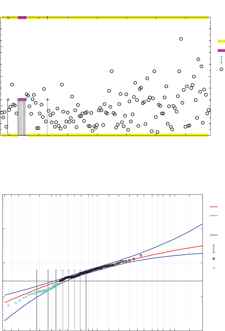
30 Flood-Frequency Estimation for Very Low Annual Exceedance Probabilities
Perception threshold,
in cubic feet per second
0 to infinity
60,000 to infinity
Censored flow
Gaged peak
1880 1900 1920 1940 1960 1980 2000
Water year
0
50,000
100,000
150,000
200,000
Annual peak streamflow, in cubic feet per second
EXPLANATION
Station 05OJ015, Red River of the North at James Avenue Pumping Station, Winnipeg, Manitoba, Canada
Figure 6. Peaks and thresholds used as input for flood-frequency analysis scenarios 1 and 2 (systematic record) for streamgage
station 05OJ015, Red River of the North at James Avenue Pumping Station, Winnipeg, Manitoba, Canada.
EXPLANATION
0.00010.010.10.5
2102550
70
909899.5
Annual exceedance probability, in percent
1,000
10,000
100,000
1,000,000
10,000,000
Annual peak streamflow, in cubic feet per second
Peakfq v 7.2 run 10/5/2019 12:25:10 PM
Expected Moments Algorithm (EMA) using
Station Skew option
−0.386 = Skew (G)
0.0541 = Mean Sq Error (MSE sub G)
Multiple Grubbs-Beck
0 Zeroes not displayed
0 Censored flows below PILF (LO) Threshold
39 Gaged peaks below PILF (LO) Threshold
Fitted frequency
Potentially influential low flood
(PILF) threshold, 29,000 cubic
feet per second
Confidence limit—5-percent lower,
95-percent upper
Censored flow
Gaged peak
PILF
Station 05OJ015, Red River of the North at James Avenue Pumping Station, Winnipeg, Manitoba, Canada
Figure 7. Annual exceedance probability plot and fitted distribution for streamgage station 05OJ015 with the input data shown in
figure 6 and at-site skew (scenario 1).

Case Study Results and Discussion 31
EXPLANATION
Perception threshold,
in cubic feet per second
0 to infinity
60,000 to infinity
106,000 to infinity
Censored flow
Interval flow
Gaged peak
Historical or paleoflood peak
1650
1700 1750
1800 1850 1900 1950 2000
Water year
0
100,000
200,000
300,000
400,000
Annual peak streamflow, in cubic feet per second
Station 05OJ015, Red River of the North at James Avenue Pumping Station, Winnipeg, Manitoba, Canada
Figure 8. Systematic and historical peaks, paleo-derived peaks, and historical and paleo-derived thresholds used for flood-frequency
analysis scenarios 9 and 10 for streamgage station 05OJ015, Red River of the North at James Avenue Pumping Station, Winnipeg,
Manitoba, Canada.
EXPLANATION
0.00010.010.10.5
2102550
70
909899.5
Annual exceedance probability, in percent
1,000
10,000
100,000
1,000,000
10,000,000
Annual peak streamflow, in cubic feet per second
Peakfq v 7.2 run 10/5/2019 12:33:25 PM
Expected Moments Algorithm (EMA) using
Station Skew option
0.0424 = Skew (G)
0.0165 = Mean Sq Error (MSE sub G)
Multiple Grubbs-Beck
0 Zeroes not displayed
0 Censored flows below PILF (LO) Threshold
39 Gaged peaks below PILF (LO) Threshold
Fitted frequency
Potentially influential low flood
(PILF) threshold, 29,000 cubic
feet per second
Confidence limit—5-percent lower,
95-percent upper
Censored flow
Interval flood estimate
Gaged peak
PILF
Historical or paleoflood peak
Station 05OJ015, Red River of the North at James Avenue Pumping Station, Winnipeg, Manitoba, Canada
Figure 9. Annual exceedance probabilities for streamgage station 05OJ015, Red River of the North at James Avenue Pumping Station,
Winnipeg, Manitoba, Canada, with the input data depicted in figure 8 and at-site skew (scenario 9).

32 Flood-Frequency Estimation for Very Low Annual Exceedance Probabilities
be the best estimate of skew for the Red River at Winnipeg
because the regional skew is based in many streamgages that
have much smaller peaks and shorter periods of record.
All scenarios are aligned along a single x-axis in gures
11–16 to compare the point estimates and 95-percent con-
dence intervals for the AEPs derived from PeakFQ. These g-
ures have an added vertical line that indicates the mean of the
point estimates. This line is not meant to indicate an ensemble
mean or other recommendation of a “best” estimate; it is sim-
ply a way to vertically compare the point estimates. Figures
12–16 feature an added vertical line indicating the point
estimate for the largest ood found to have occurred in over
350 years, 225,000 ft
3
/s in 1826. Figure 12 also shows point
estimates from other studies discussed in the next section.
Comparisons to Other Flood-Frequency Methods
Burn and Goel (2001) published ood-frequency analysis
for the Red River at Winnipeg using the gaged record through
1998 (naturalized by Manitoba Water Stewardship as was
the data we used), the three historical peaks from the Canada
Department of Resources and Development (1953), and histor-
ical peaks from Rannie (1998). Burn and Goel’s methods did
not incorporate interval estimates; therefore, they converted
the interval estimates to point estimates selected to “span the
range of ood events identied by Rannie” (Burn and Goel,
2001, p. 356; see also table 2 of Burn and Goel, 2001). Burn
and Goel (2001) found STP (lag-one serial correlation) and
LTP (signicant Hurst coecient) in the Red River record and
published ood-frequency analyses using several dierent dis-
tributions (generalized extreme value, PE3, and 3-parameter
lognormal) and estimation methods (method of moments,
MLE, and L-moments). (See Asquith and others [2017] for
details about the eect of distribution and estimation choices
on ood-frequency analysis.) Burn and Goal also used a
mixed-noise model (Booy and Lye, 1989) that generated
serially correlated data and compared it to an analysis with an
independent dataset, focusing on oods with an AEP of 0.01
(their results have been included in table 4 for comparison to
PeakFQ estimates; scenarios 11–21).
Harden (1999) reported ood-frequency results using the
PE3 distribution tted with the method of moments for several
AEPs (an AEP of 0.01 is the only one in common with this
study). Flood-frequencies were reported under ve scenarios,
three of which were included in table 4 (scenarios 22–24).
Those three include using the gaged record, the gaged record
plus four historical peaks, and the gaged record plus four
historical peaks and Rannie’s interval peaks converted to the
midpoint of Rannie’s range. Three of the historical peaks were
those determined by the Canada Department of Resources
and Development (1953) and used in our study, as well as
the study by Burn and Goel (2001). The fourth event was
described in 1776 (Rannie, 1998) but has a great deal of uncer-
tainty surrounding it. Harden (1999) used a value that was
slightly higher than the 1826 ood. However, the 1776 ood
does not appear in the tree-ring record and, therefore, was not
used in this study.
EXPLANATION
0.00010.010.10.5
2102550
70
909899.5
1,000
10,000
100,000
1,000,000
Annual peak streamflow, in cubic feet per second
Peakfq v 7.2 run 10/5/2019 12:36:57 PM
Expected Moments Algorithm (EMA) using
Weighted Skew option
−0.2 = Skew (G)
Multiple Grubbs-Beck
0 Zeroes not displayed
0 Censored flows below PILF (LO) Threshold
39 Gaged peaks below PILF (LO) Threshold
Annual exceedance probability, in percent
Fitted frequency
Potentially influential low flood
(PILF) threshold
Confidence limit—5-percent lower,
95-percent upper
Censored flow
Gaged peak
PILF
Historical or paleoflood peak
Station 05OJ015, Red River of the North at James Avenue Pumping Station, Winnipeg, Manitoba, Canada
Figure 10. Annual exceedance probabilities for streamgage station 05OJ015, Red River of the North at James Avenue Pumping
Station, Winnipeg, Manitoba, Canada, with the input data depicted in figure 8 and weighted skew (scenario 10).

Case Study Results and Discussion 33
Streamflow, in cubic feet per second
0 50,000 100,000 150,000 200,000
Scenario 1
Scenario 2
Scenario 3
Scenario 4
Scenario 5
Scenario 6
Scenario 7
Scenario 8
Scenario 9
Scenario 10
[Annual exceedance probability = 0.10]
PeakFQ point estimate
PeakFQ 95-percent confidence
interval
Mean of all point estimates,
84,308 cubic feet per second
●
●
●
●
●
●
●
●
●
●
●
EXPLANATION
Station 05OJ015, Red River of the North at James Avenue Pumping Station, Winnipeg, Manitoba, Canada
Figure 11. Point and interval estimates for streamgage station 05OJ015, Red River of the North at James Avenue Pumping Station,
Winnipeg, Manitoba, Canada, floods with annual exceedance probability of 0.10, calculated using U.S. Geological Survey PeakFQ
software (Veilleux and others, 2014) version 7.2 under 10 different scenarios. See table 4 for descriptions of the scenarios and the
numeric values.
Streamflow, in cubic feet per second
0 100,000 200,000 300,000 400,000
Scenario 1
Scenario 2
Scenario 3
Scenario 4
Scenario 5
Scenario 6
Scenario 7
Scenario 8
Scenario 9
Scenario 10
Scenario 11
Scenario 12
Scenario 13
Scenario 14
Scenario 15
Scenario 16
Scenario 17
Scenario 18
Scenario 19
Scenario 20
Scenario 21
Scenario 22
Scenario 23
Scenario 24
●
●
●
●
●
●
●
●
●
●
Peak estimate from Burn and Goel (2001)
Peak estimate from Harden (1999)
Largest flood in over 350 years (1826),
225,000 cubic feet per second
[Annual exceedance probability = 0.01]
PeakFQ 95-percent confidence interval
Mean of all point estimates,
141,200 cubic feet per second
PeakFQ point estimate
●
EXPLANATION
Station 05OJ015, Red River of the North at James Avenue Pumping Station, Winnipeg, Manitoba, Canada
Figure 12. Point and interval estimates for streamgage station 05OJ015, Red River of the North at James Avenue Pumping
Station, Winnipeg, Manitoba, Canada, floods with annual exceedance probability of 0.01, calculated using U.S. Geological Survey
PeakFQ software (Veilleux and others, 2014) version 7.2 under 10 different scenarios and 13 additional point estimates from other
flood-frequency studies (Burn and Goel, 2001; Harden, 1999). See table 4 for descriptions of the scenarios and the numeric values.

34 Flood-Frequency Estimation for Very Low Annual Exceedance Probabilities
Streamflow, in cubic feet per second
0 100,000 200,000 300,000 400,000 500,000
Scenario 1
Scenario 2
Scenario 3
Scenario 4
Scenario 5
Scenario 6
Scenario 7
Scenario 8
Scenario 9
Scenario 10
●
●
●
●
●
●
●
●
●
●
Largest flood in over 350 years (1826),
225,000 cubic feet per second
[Annual exceedance probability = 1×10
−3
]
PeakFQ 95-percent confidence interval
Mean of all point estimates,
189,630 cubic feet per second
PeakFQ point estimate
●
EXPLANATION
Station 05OJ015, Red River of the North at James Avenue Pumping Station, Winnipeg, Manitoba, Canada
Figure 13. Point and interval estimates for streamgage station 05OJ015, Red River of the North at James Avenue Pumping Station,
Winnipeg, Manitoba, Canada, floods with annual exceedance probability of 1×10
−3
, calculated using U.S. Geological Survey PeakFQ
software (Veilleux and others, 2014) version 7.2 under 10 different scenarios. See table 4 for descriptions of the scenarios and the
numeric values.
Streamflow, in cubic feet per second
0
250,000 500,000 750,000 1,000,000 1,250,000
Scenario 1
Scenario 2
Scenario 3
Scenario 4
Scenario 5
Scenario 6
Scenario 7
Scenario 8
Scenario 9
Scenario 10
●
●
●
●
●
●
●
●
●
●
Largest flood in over 350 years (1826),
225,000 cubic feet per second
[Annual exceedance probability = 1×10
−4
]
PeakFQ 95-percent confidence interval
Mean of all point estimates,
247,760 cubic feet per second
PeakFQ point estimate
●
EXPLANATION
Station 05OJ015, Red River of the North at James Avenue Pumping Station, Winnipeg, Manitoba, Canada
Figure 14. Point and interval estimates for streamgage station 05OJ015, Red River of the North at James Avenue Pumping Station,
Winnipeg, Manitoba, Canada, floods with annual exceedance probability of 1×10
−4
, calculated using U.S. Geological Survey PeakFQ
software (Veilleux and others, 2014) version 7.2 under 10 different scenarios. See table 4 for descriptions of the scenarios and the
numeric values.

Case Study Results and Discussion 35
Streamflow, in cubic feet per second
0
250,000 500,000 750,000 1,000,000 1,250,000 1,500,000 1,750,000 2,000,000 2,250,000
Scenario 1
Scenario 2
Scenario 3
Scenario 4
Scenario 5
Scenario 6
Scenario 7
Scenario 8
Scenario 9
Scenario 10
●
●
●
●
●
●
●
●
●
●
Largest flood in over 350 years (1826),
225,000 cubic feet per second
[Annual exceedance probability = 1×10
−5
]
PeakFQ 95-percent confidence interval
Mean of all point estimates,
313,500 cubic feet per second
PeakFQ point estimate
●
EXPLANATION
Station 05OJ015, Red River of the North at James Avenue Pumping Station, Winnipeg, Manitoba, Canada
Figure 15. Point and interval estimates for streamgage station 05OJ015, Red River of the North at James Avenue Pumping Station,
Winnipeg, Manitoba, Canada, floods with annual exceedance probability of 1×10
−5
, calculated using U.S. Geological Survey PeakFQ
software (Veilleux and others, 2014) version 7.2 under 10 different scenarios. See table 4 for descriptions of the scenarios and the
numeric values.
Streamflow, in cubic feet per second
0
1,000,000 2,000,000 3,000,000 4,000,000 5,000,000
Scenario 1
Scenario 2
Scenario 3
Scenario 4
Scenario 5
Scenario 6
Scenario 7
Scenario 8
Scenario 9
Scenario 10
Infinite bound
●
●
●
●
●
●
●
●
●
●
Largest flood in over 350 years (1826),
225,000 cubic feet per second
[Annual exceedance probability = 1×10
−6
]
PeakFQ 95-percent confidence
interval
Mean of all point estimates,
388,700 cubic feet per second
PeakFQ point estimate
●
EXPLANATION
Station 05OJ015, Red River of the North at James Avenue Pumping Station, Winnipeg, Manitoba, Canada
Figure 16. Point and interval estimates for streamgage station 05OJ015, Red River of the North at James Avenue Pumping Station,
Winnipeg, Manitoba, Canada, floods with annual exceedance probability of 1×10
−6
, calculated using U.S. Geological Survey PeakFQ
software (Veilleux and others, 2014) version 7.2 under 10 different scenarios. See table 4 for descriptions of the scenarios and the
numeric values.
36 Flood-Frequency Estimation for Very Low Annual Exceedance Probabilities
Summary
The peak-ow record for the Red River at Winnipeg
exhibits autocorrelation, a change point, and a monotonic
trend. These are all nonstationarities, and Federal guidance
does not yet exist for how to deal with these. Major implica-
tions for the autocorrelation include that trend analysis may
report incorrect p-values and that there is redundancy in the
record. When the MKT was modied to deal with serial cor-
relation, the trend was still signicant. When historical and
paleoood information is added to the record, this extends
the record and provides additional information for the upper
end of the distribution, osetting the shortening of the eec-
tive record from autocorrelation. The identication of PILFs
decreases the eect of some of the peaks in the drier period,
which helps to address the change point.
The addition of regional information by using a skew
weighted with regional information did not improve the t of
the distribution to the low AEP oods. Regional skew may not
be the best estimate of skew for this site because the regional
skew is based in many streamgages that have much smaller
peaks and shorter periods of record. Historical and paleoood
data add information to the upper end of the ood-frequency
distribution and provide more information for estimating very
low AEP oods.
For AEPs of 0.10 (g. 11 and table 4), compared to the
full systematic record (scenarios 1 and 2), adding historical
and paleoood data and associated thresholds (scenarios 9
and 10) slightly decreases the ood estimates and the widths
for the condence bounds. Scenario 5 (using the most recent
30 years of record, assuming it is indicative of future condi-
tions) has a much larger point estimate than the other scenarios
and much wider condence bounds. This is likely because of
the serial correlation in the data, resulting in a record of less
than 30 years and a great deal of uncertainty.
The graphical depiction of the estimates for the AEP
of 0.01 (g. 12) highlights dierences in the estimates and
condence interval widths as more information is added to the
analysis and dierent periods are used. Compared to using the
systematic record with at-site skew (scenario 1), the addition
of paleoood and historical estimates and thresholds increases
the 0.01 AEP estimates and decreases the condence interval
widths (scenario 9), showing the precision benet of including
additional information about ood magnitude and frequency.
The largest point estimates, in decreasing order, are the most
recent 30 years with EMA–PE3 (scenario 5, 161,000 ft
3
/s),
Harden’s 1999 analysis using the systematic record plus his-
torical peaks (scenario 23, 157,000 ft
3
/s), the systematic peaks
plus historical peaks (scenario 7, 156,000 ft
3
/s), and Burn and
Goel’s 2001 mixed-noise model (scenario 20, 154,000 ft
3
/s).
Condence bounds are not available for the other studies
but for those determined with EMA–PE3 (scenarios 1–10),
scenario 5 is noticeable for wide condence bounds. Two
scenarios, 7 and 23, show how adding historical peaks (with-
out longer term paleoood data) has the potential to bias the
ood estimate up. Scenario 23 was based on the addition of
four large historical peaks (one of them with a great deal of
uncertainty) and no paleoood data, so it is reasonable to think
of this as potentially being biased high.
Scenarios 9 (systematic, historical, and paleoood with
at-site skew), 10 (systematic, historical, and paleoood with
weighted skew), and 20 (Burn and Goel, 2001; mixed-noise
model that addresses the correlation in the series) seem the
most realistic. Booy and Morgan (1985) used a fractional-
noise model and Bayesian updating to show that the clustering
of oods in the Red River record results in underestimates of
ood risk for Winnipeg when the series is analyzed with meth-
ods that assume independence. The estimate from scenario 20
that address the correlation is within the condence intervals
for scenarios 9 and 10 (g. 12). For this site, the addition of
historical and paleoood peaks and thresholds extend the
record, osetting the loss of information in a correlated series.
Figure 13 shows a distinct dierence between those sce-
narios that have historical or paleoood information (scenar-
ios 7–10) and those that do not (scenarios 1–6), with the mean
estimates for an AEP of 1×10
−3
being above the overall mean
point estimate for scenarios 7–10 and below the overall mean
for scenarios 1–6. Adding only the historical peaks and thresh-
olds results in large estimates with wide condence intervals.
Providing additional magnitude and frequency information
with additional paleoood data reduces the point estimates and
the width of the condence intervals. According to scenario 9
(systematic, historical, and paleoood with at-site skew), the
1826 ood has an AEP of approximately 1×10
−3
. If only the
systematic data were used (scenario 1), gure 14 indicates that
the 1826 ood would have an approximate an AEP of 1×10
−4
.
Figures 15 and 16 further emphasize the dierences in
point estimates generated using systematic data or generated
with systematic data and historical or paleoood data. The
gures also highlight some dramatic dierences in condence
bounds for an AEP of 1×10
−5
and 1×10
−6
. If one desires to
extend the record with estimates of peaks beyond the system-
atic record, historical and paleoood data seem necessary to
produce more precise condence intervals.
Comparison of methods and AEPs in gures 15 and 16
shows that there is a great deal of variability among estimates,
depending on the period of record used, on whether histori-
cal and paleoood data are used, on the AEP being estimated,
and on the skew used. Using the dry period only (scenario 3)
underestimates the potential ood, and as the AEP becomes
smaller, the dry period estimate has wider condence bounds.
Using the most recent 30 years of data (scenario 5) seems to
bias the ood to the larger end when the AEP is 0.10 or 0.01
and results in huge condence intervals as AEPs become
smaller, which is understandable given 30 years of record
is too short to reliably estimate very low AEP oods. The
ood-frequency analysis that incorporated the mean-shifted
dry period (scenario 6) has narrower condence intervals than
many of the other estimates, which is logical in that the shift
reduced the variability in the underlying data. Adding histori-
cal peaks and thresholds (scenarios 7 and 8) to the systematic
record tends to increase the condence interval, which is
Case Study Results and Discussion 37
reasonable given that historical peaks are usually biased large
and would aect the ood-frequency curve. However, by add-
ing paleoood peaks and thresholds (scenarios 9 and 10) that
provide a longer-term description of the occurrence of very
large oods, the condence interval can narrow. The choice of
skew also makes a signicant dierence in the point estimates
and the width of the condence intervals. For this case study
and the given set of the data, the weighted skew generally
gives lower point estimates and narrower condence intervals
than at-site skew; however, on the basis of visual inspection of
the t, at-site skew produces a distribution that better ts the
peaks at the upper end of the distribution.
The eects of moving from an analysis with the system-
atic record to an analysis with a record that includes historical
and paleoood peaks and thresholds (including regional infor-
mation in the form of a weighted skew) are shown in gures
17 and 18. Figure 17 shows the point and interval estimates,
for a range of annual exceedance probabilities, resulting from
ood-frequency analysis with the systematic record only using
at-site (scenario 1; g. 17A) and weighted skew (scenario 2;
g. 17B; table 4). Figure 18 shows the point and interval
estimates, for a range of annual exceedance probabilities,
resulting from ood-frequency analysis with systematic and
historical peaks, historical and paleo-derived estimates, and
paleo-derived thresholds, using at-site (scenario 9; g. 18A)
and weighted skew (scenario 10; g. 18B; table 4). Again,
the systematic record indicates the 1826 ood has an AEP
of approximately 1×10
−4
. However, when additional his-
torical and paleoood information is added, the 1826 ood
becomes more likely with an AEP of approximately 1×10
−3
.
Using weighted skew reduces the point estimates for all ood
quantiles except those with AEPs of 0.10 and results in more
precise condence bounds for the lowest AEPs.

38 Flood-Frequency Estimation for Very Low Annual Exceedance Probabilities
Streamflow, in cubic feet per second
0
250,000 500,000 750,000 1,000,000
81,750 cubic feet per second, annual exceedance probability = 0.10
132,800 cubic feet per second, annual exceedance probability = 0.01
180,700 cubic feet per second, annual exceedance probability = 1×10
−3
226,400 cubic feet per second, annual exceedance probability = 1×10
−4
270,000 cubic feet per second, annual exceedance probability = 1×10
−5
311,300 cubic feet per second, annual exceedance probability = 1×10
−6
Upper bound is 1,364,000 cubic feet
per second
Streamflow, in cubic feet per second
0
250,000 500,000 750,000 1,000,000
81,740 cubic feet per second, annual exceedance probability = 0.10
130,100 cubic feet per second, annual exceedance probability = 0.01
173,000 cubic feet per second, annual exceedance probability = 1×10
−3
211,800 cubic feet per second, annual exceedance probability = 1×10
−4
246,800 cubic feet per second, annual exceedance probability = 1×10
−5
278,400 cubic feet per second, annual exceedance probability = 1×10
−6
●
●
●
●
●
●
●
●
●
●
●
●
Largest flood in over 350 years (1826),
225,000 cubic feet per second
[Systematic record, weighted skew]
PeakFQ 95-percent confidence interval
PeakFQ point estimate
●
EXPLANATION
A. Scenario 1
B. Scenario 2
Largest flood in over 350 years (1826),
225,000 cubic feet per second
[Systematic record, site skew]
PeakFQ 95-percent confidence interval
Upper bound extends beyond
x-axis scale
PeakFQ point estimate
●
EXPLANATION
Station 05OJ015, Red River of the North at James Avenue Pumping Station, Winnipeg, Manitoba, Canada
Figure 17. Point and interval estimates for a range of annual exceedance probabilities for streamgage station 05OJ015, Red River of
the North at James Avenue Pumping Station, Winnipeg, Manitoba, Canada, floods, calculated using U.S. Geological Survey PeakFQ
software (Veilleux and others, 2014) version 7.2, with A, at-site and B, weighted skew and the systematic record only. This depicts
analysis results for A, scenario 1 and B, scenario 2 of table 4.

Case Study Results and Discussion 39
A. Scenario 9
B. Scenario 10
Largest flood in over 350 years (1826),
225,000 cubic feet per second
[Systematic record, site skew]
PeakFQ 95-percent confidence interval
Upper bound extends beyond
x-axis scale
PeakFQ point estimate
●
EXPLANATION
Largest flood in over 350 years (1826),
225,000 cubic feet per second
[Systematic record, weighted skew]
PeakFQ 95-percent confidence interval
PeakFQ point estimate
●
EXPLANATION
Streamflow, in cubic feet per second
0
250,000 500,000 750,000 1,000,000
78,020 cubic feet per second, annual exceedance probability = 0.10
140,800 cubic feet per second, annual exceedance probability = 0.01
218,000 cubic feet per second, annual exceedance probability = 1×10
−3
313,400 cubic feet per second, annual exceedance probability = 1×10
−4
430,700 cubic feet per second, annual exceedance probability = 1×10
−5
572,700 cubic feet per second, annual exceedance probability = 1×10
−6
Upper bound is 2,112,000 cubic feet
per second
Upper bound is 1,164,000 cubic feet
per second
Streamflow, in cubic feet per second
0
250,000 500,000 750,000 1,000,000
78,810 cubic feet per second, annual exceedance probability = 0.10
135,300 cubic feet per second, annual exceedance probability = 0.01
195,800 cubic feet per second, annual exceedance probability = 1×10
−3
261,400 cubic feet per second, annual exceedance probability = 1×10
−4
332,000 cubic feet per second, annual exceedance probability = 1×10
−5
407,200 cubic feet per second, annual exceedance probability = 1×10
−6
●
●
●
●
●
●
●
●
●
●
●
●
Station 05OJ015, Red River of the North at James Avenue Pumping Station, Winnipeg, Manitoba, Canada
Figure 18. Point and interval estimates for a range of annual exceedance probabilities for streamgage station 05OJ015, Red River
of the North at James Avenue Pumping Station, Winnipeg, Manitoba, Canada, floods, calculated using U.S. Geological Survey
PeakFQ software version 7.2 with A, at-site and B, weighted skew and the systematic record plus historical peaks and thresholds and
paleo-derived peaks and paleo-derived thresholds. This depicts analysis results for A, scenario 9 and B, scenario 10 of table 4.

40 Flood-Frequency Estimation for Very Low Annual Exceedance Probabilities
Lower reach, Rapid Creek, South Dakota
The peak-ow record for the lower reach of Rapid Creek
is based on streamow records from multiple streamgages
that were compiled and adjusted to be comparable with a
paleoood chronology developed for this reach (Harden and
others, 2011). This synthetic record is referred to as a system-
atic record for consistency with the other case studies because
the synthetic record is based on systematic record collection.
Some peaks were designated as historical. The historical and
systematic peaks are depicted in gure 19.
Initial Data Analysis
For the autocorrelation analysis, only the systemic record
(1929–2009) peak series was examined. Figure 20 shows
that this site does not have autocorrelation. In gure 21, the
change-point algorithm assumes all peaks are consecutive
(that is why the historical and paleoood point estimates were
not included) and relabels them 1 to n, where n is the number
of values in the series. Figure 21 shows that the high outlier
(1972) peak causes a change point, highlighting the challenge
of determining reasonable criteria for change points given
outliers. When the historical peaks are included, there is a
downward trend in peak ow; however, when those peaks are
not included, there is no trend in peak ow (g. 22).
Flood-Frequency Analysis
Flood-frequency analysis with at-site skew was originally
considered, but the t (not shown) was very poor. Therefore,
ood-frequency analysis was analyzed under three scenarios,
with comparisons to seven other variations on ood-frequency
analysis from a previous study:
1. systematic peaks, with weighted skew;
2. systematic peaks and historical peaks, with
weighted skew;
3. systematic data, historical peaks, and paleo-derived
interval peaks and thresholds, with weighted skew;
4–10. in addition to the analyses performed for this study,
estimates were obtained from another ood-frequency
study (Harden and others, 2011) and are presented as
comparison scenarios. See table 5 (available for down-
load at https://doi.org/ 10.3133/ sir20205065) for more
information.
The historical peaks under 7,000 ft
3
/s were designated
opportunistic and not included in the ood-frequency analy-
sis. The peaks not designated as historical, but outside a
systematic period of record, did not t the distribution of
the other peaks. Therefore, they were treated as opportunis-
tic peaks (Sando and McCarthy, 2018) and removed. Sando
(1998) found that the generalized skew coecient from
the map in Bulletin 17B (U.S. Water Resources Council,
Annual peak streamflow, in cubic feet per second
10
100
1,000
10,000
100,000
1875 1900 1925 1950 1975 2000 2025
Water year
●
●
●
●
●
●
●
●
●
●
●
●
●
●
●
●
●
●
●
●
●
●
●
●
●
●
●
●
●
●
●
●
●
●
●
●
●
●
●
●
●
●
●
●
●
●
●
●
●
●
●
●
●
●
●
●
●
●
●
●
●
●
●
●
●
●
●
●
●
●
●
●
●
●
●
●
●
●
●
●
●
EXPLANATION
Historical peak
Systematic peak
●
Lower reach, Rapid Creek, South Dakota
Figure 19. Systematic peaks and historical peaks for lower reach, Rapid Creek, South Dakota (Harden and others,
2011).
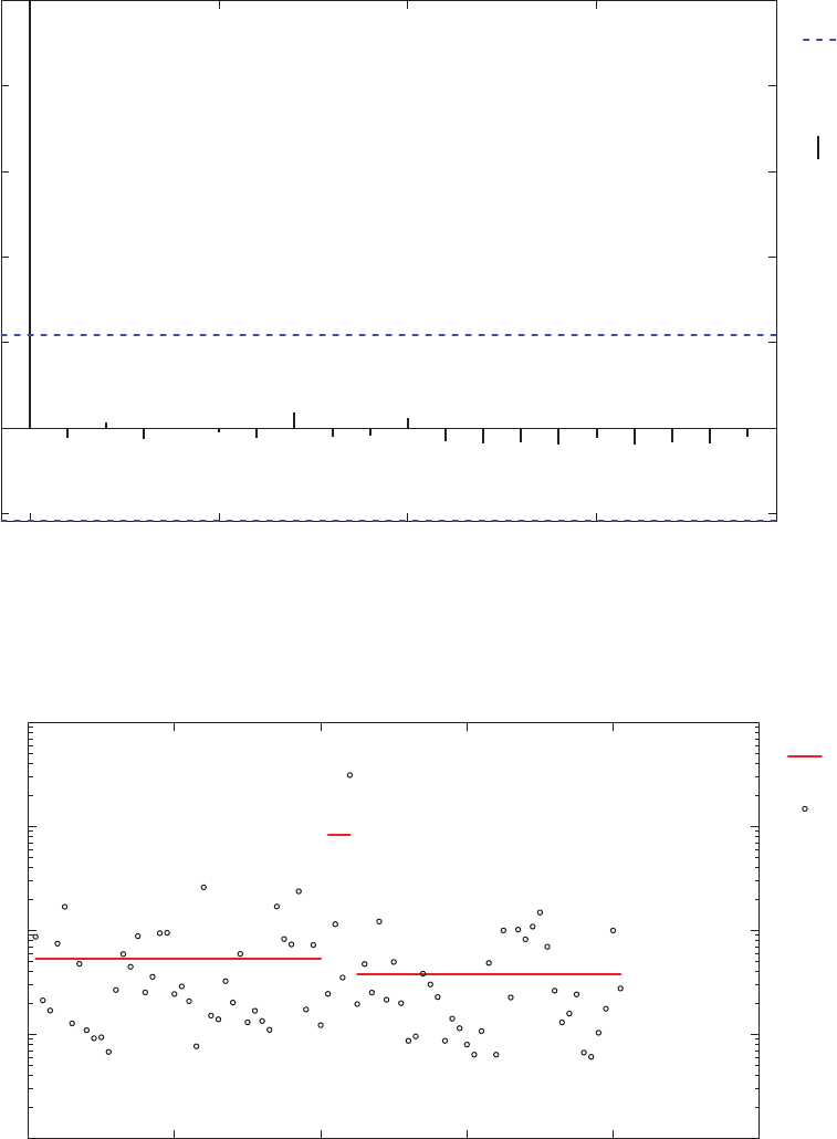
Case Study Results and Discussion 41
0 5 10 15
−0.2
0
0.2
0.4
0.6
0.8
1.0
Lag, in water years (all peaks treated as consecutive)
Autocorrelation
Line of statistical significance—
Autocorrelations that cross
these lines are statistically
significant at a 0.05
significance level
Autocorrelation
EXPLANATION
Lower reach, Rapid Creek, South Dakota
Figure 20. The autocorrelation for peaks in systematic period of record for lower reach, Rapid Creek, South Dakota.
EXPLANATION
Observation (all peaks treated as consecutive)
Annual peak streamflow, in cubic feet per second
0 20 40 60 80 100
10
100
1,000
10,000
100,000
●
●
●
●
●
●
●
●
●
●
●
●
●
●
●
●
●
●
●
●
●
●
●
●
●
●
●
●
●
●
●
●
●
●
●
●
●
●
●
●
●
●
●
●
●
●
●
●
●
●
●
●
●
●
●
●
●
●
●
●
●
●
●
●
●
●
●
●
●
●
●
●
●
●
●
●
●
●
●
●
●
●
Lower reach, Rapid Creek, South Dakota
Mean of distribution of
annual peak streamflow
Annual peak streamflow
Figure 21. Change points in mean and variance for peaks in systematic period of record for lower reach, Rapid Creek, South
Dakota.

42 Flood-Frequency Estimation for Very Low Annual Exceedance Probabilities
1976) was adequate for South Dakota streamgages; therefore,
the regional skew used was 0.194 with a mean square error
of 0.302.
Given the magnitude of the 1972 peak, which was con-
siderably larger than any other peak in the systematic or his-
torical record, the ood-frequency curves for systematic data
only and systematic plus historical data did not completely
plot in PeakFQ because of the steep slope and extremely
large condence bounds on the very low AEPs and are not
shown. The input information and the resulting ood-
frequency curve for scenario 3 are shown in gures 23 and 24,
and selected AEPs for the three scenarios are shown in table 5.
Comparisons to Other Flood-Frequency Methods
Harden and others (2011) completed ood-frequency
analysis with several techniques using the same dataset with
the exception that they used the opportunistic peaks in some
analyses. As compared to some other ood-frequency meth-
ods used for comparisons to results at other sites in this study,
the methods used by Harden and others (2011) were able to
incorporate paleoood data, including interval estimates and
thresholds, and they provided condence intervals for their
estimates. They used two models that used PE3 distributions:
FLDFRQ3 (O’Connell, 1999; O’Connell and others, 2002)
and PeakfqSA (Cohn and others, 1997; Cohn and others, 2001;
Gris and others, 2004). FLDFRQ3 uses a Bayesian approach
described in O’Connell and others (2002) with MLE. Results
from Harden and others (2011) under seven dierent sce-
narios are shown in table 5 and designated as scenarios 4–10.
Scenarios 4–7 use PeakfqSA and 8–10 use FLDFRQ3.
For an AEP of 0.01, all 10 scenarios are plotted in
gure 25 to compare the estimates. Scenarios 1, 4, and 8
are very similar in that they use the same data (except for
the opportunistic peaks dropped in this study). Scenarios 4
and 8 have much larger condence intervals, presumably
because of the four extra peaks used that do not t well with
the distribution of other peaks. Scenarios 2, 5, and 9 are also
very similar (except for the opportunistic peaks). Scenario 5,
using PeaksfqSA, has much larger condence bounds than
scenarios 2 and 9. Scenarios 3, 6, and 10 also use similar
data (except for the opportunistic peaks) and produce similar
estimates and condence bounds. Scenario 7 uses top tting
by excluding peak values less than the median and produces
the largest estimate for an AEP of 0.01.
Summary
The peak-ow record for the lower reach of Rapid Creek
is not autocorrelated. The large 1972 peak causes a change
point in the distribution if one uses a fairly short minimum
segment length for change points (four in this analysis).
This highlights the challenge in dening change points. The
1972 peak would have a large eect on moving means and
variances that include this peak; therefore, one may want to
treat the 1972 peak as an outlier rather than a change point.
Change point detections are not denitive because of the many
methods and criteria that can be adjusted. Statistical analysis
should include graphical analysis (such as g. 21) that allow
one to place the change point(s) in context with what is known
about the hydroclimatology and setting of the streamgage site.
EXPLANATION
Mann-Kendall trend line for
systematic record and
historical peaks, p-value=0.01
Mann-Kendall trend line for
systematic record, p
-value=0.33
●
1880 1900 1920 1940 1960 1980 2000 2020
Annual peak streamflow, in cubic feet per second
10
100
1,000
10,000
100,000
●
●
●
●
●
●
●
●
●
●
●
●
●
●
●
●
●
●
●
●
●
●
●
●
●
●
●
●
●
●
●
●
●
●
●
●
●
●
●
●
●
●
●
●
●
●
●
●
●
●
●
●
●
●
●
●
●
●
●
●
●
●
●
●
●
●
●
●
●
●
●
●
●
●
●
●
●
●
●
●
●
Trend lines
Lower reach, Rapid Creek, South Dakota
Annual peak streamflow
Historical peak
Figure 22. Mann-Kendall test for trend in the peak-streamflow record for lower reach, Rapid Creek, South Dakota.

Case Study Results and Discussion 43
EXPLANATION
Perception threshold, in
cubic feet per second
0 to infinity
7,000 to infinity
9,500 to infinity
64,000 to infinity
79,000 to infinity
Censored flow
Interval flow
Gaged peak
Historical peak
800 1000
1200 1400
1600 1800 2000
Water year
0
50,000
100,000
150,000
200,000
Annual peak streamflow, in cubic feet per second
Lower reach, Rapid Creek, South Dakota
Figure 23. Systematic and historical peaks, paleo-derived interval peaks, and historical and paleo-derived thresholds used as
input for flood-frequency analysis with weighted skew (scenario 3), lower reach, Rapid Creek, South Dakota.
EXPLANATION
0.00010.010.1
1520
40
70
909899.5
Annual exceedance probability, in percent
10
100
1,000
10,000
100,000
1,000,000
10,000,000
100,000,000
Annual peak streamflow, in cubic feet per second
Peakfq v 7.2 run 10/5/2019 1:53:13 PM
Expected Moments Algorithm (EMA) using
Weighted Skew option
0.407 = Skew (G)
Multiple Grubbs-Beck
0 Zeroes not displayed
0 Censored flows below PILF (LO) Threshold
0 Gaged peaks below PILF (LO) Threshold
Fitted frequency
Confidence limit—5-percent lower,
95-percent upper
Censored flow
Interval flood estimate
Gaged peak
Historical peak
Lower reach, Rapid Creek, South Dakota
Figure 24. Annual exceedance probability plot and fitted distribution for lower reach of Rapid Creek, South Dakota, using the input
data depicted in figure 23 and weighted skew (scenario 3).

44 Flood-Frequency Estimation for Very Low Annual Exceedance Probabilities
When including early historical peaks, there is a statistically
signicant downward trend for the lower reach of Rapid Creek
(g. 22). This means that AEP estimates may be biased high,
given current conditions, but cannot be extrapolated to future
conditions.
Using a skew weighted with regional information
greatly improved the t of the distribution to the low AEP
oods. This site is a special case in that it has a high outlier
in the gaged record and large paleoood peaks. The paleo-
ood peaks do help provide context for the outlier peak and
improve the t of the distribution. These large peaks result in
a steep ood-frequency curve with large error bounds when
estimating very low AEPs. Fewer scenario comparisons were
plotted for this site than others in the study because the error
bounds are so large that it is dicult to graphically compare
the results. The complete set of AEPs estimated in this study,
along with condence bounds, are plotted in gures 26 and 27
for the three scenarios that were estimated using EMA–PE3
(scenarios 1–3).
Using paleoood data results in a substantial reduction
in the condence bounds for very low AEPs; however, the
bounds remain large for very low AEPs (less than 0.001).
This jointly highlights the value of paleoood data and the
challenge of obtaining precise magnitude estimates for very
low AEPs.
Streamflow, in cubic feet per second
0
40,000 80,000 120,000
Scenario 1
Scenario 2
Scenario 3
Scenario 4
Scenario 5
Scenario 6
Scenario 7
Scenario 8
Scenario 9
Scenario 10
●
●
●
●
●
●
●
●
●
●
[Annual exceedance probability = 0.01]
PeakFQ 95-percent confidence interval
Mean of all point estimates,
11,416 cubic feet per second
PeakFQ point estimate
●
EXPLANATION
Lower reach, Rapid Creek, South Dakota
Figure 25. Point estimates and confidence bounds for scenarios using U.S. Geological Survey PeakFQ software (Veilleux and others,
2014) version 7.2 for lower reach of Rapid Creek, South Dakota, for floods with annual exceedance probability of 0.01, calculated under
three different PeakFQ scenarios and compared to seven estimates from Harden and others (2011). See table 5 for descriptions of the
scenarios and the numeric values.

Case Study Results and Discussion 45
[Systematic data]
PeakFQ 95-percent confidence interval
Upper bound extends beyond
x-axis scale
PeakFQ point estimate
●
EXPLANATION
[Systematic data]
PeakFQ 95-percent confidence interval
Upper bound extends beyond
x-axis scale
PeakFQ point estimate
●
EXPLANATION
A. Scenario 1
B. Scenario 2
Streamflow, in cubic feet per second
0 1,000,000 2,000,000 3,000,000 4,000,000 5,000,000
1,323 cubic feet per second, annual exceedance probability = 0.10
7,156 cubic feet per second, annual exceedance probability = 0.01
30,880 cubic feet per second, annual exceedance probability = 1×10
−3
119,600 cubic feet per second, annual exceedance probability = 1×10
−4
433,300 cubic feet per second, annual exceedance probability = 1×10
−5
1,493,000 cubic feet per second, annual exceedance probability = 1×10
−6
Upper bound is 7,572,000 cubic feet
per second
Upper bound is 116,300,000 cubic feet
per second
Upper bound is 1,749,000,000 cubic feet
per second
Streamflow, in cubic feet per second
0 1,000,000 2,000,000 3,000,000 4,000,000 5,000,000
1,775 cubic feet per second, annual exceedance probability = 0.10
10,960 cubic feet per second, annual exceedance probability = 0.01
51,730 cubic feet per second, annual exceedance probability = 1×10
−3
214,700 cubic feet per second, annual exceedance probability = 1×10
−4
823,500 cubic feet per second, annual exceedance probability = 1×10
−5
2,976,000 cubic feet per second, annual exceedance probability = 1×10
−6
Upper bound is 6,157,000 cubic feet
per second
Upper bound is 79,380,000 cubic feet
per second
Upper bound is 1,003,000,000 cubic feet
per second
●
●
●
●
●
●
●
●
●
●
●
●
Lower reach, Rapid Creek, South Dakota
Figure 26. Point and interval estimates for a range of annual exceedance probabilities for lower reach of Rapid Creek, South Dakota,
floods, calculated using U.S. Geological Survey PeakFQ software (Veilleux and others, 2014) version 7.2 with A, as weighted skew and
systematic data and B, as systematic plus historical data. This depicts A, as scenario 1 and B, as scenario 2 of table 5.

46 Flood-Frequency Estimation for Very Low Annual Exceedance Probabilities
Spring Creek, South Dakota
The peak-ow record for Spring Creek is based on
streamow records from multiple streamgages that were com-
piled and adjusted to be comparable with a paleoood chro-
nology developed for this reach (Harden and others, 2011).
This synthetic record is referred to as a systematic record for
consistency with the other case studies because the synthetic
record is based on systematic record collection. More infor-
mation about this site and the paleoood data is available in
Harden and others (2011).
Initial Data Analysis
The systematic peaks were examined for autocorrelation,
change points, and a trend. There is no autocorrelation at this
site (g. 28), but there a several change points in the mean
and variance (g. 29). Most notable is the largest ood in the
record (the 1972 ood), which causes a change in the mean
and variance. Despite changes in mean and variance, there is
no trend over the period of systematic record (g. 30).
Flood-Frequency Analysis
Flood-frequency analysis with at-site skew was originally
considered, but the t (not shown) was very poor. Therefore,
ood-frequency analysis was performed under three scenarios,
with comparisons to two other variations on ood-frequency
analysis from a previous study:
1. systematic peaks, with weighted skew;
2. systematic peaks with paleo-derived peaks and thresh-
olds, with weighted skew;
3. systematic peaks with predicted paleo-derived peaks
and thresholds on the basis of paleooods in the nearby
lower reach of Rapid Creek, with weighted skew;
4–5. in addition to the analyses performed for this study,
estimates were obtained from another ood-frequency
study (Harden and others, 2011) and are presented as
comparison scenarios. See table 6 (available for down-
load at https://doi.org/ 10.3133/ sir20205065) for more
information.
There were peaks in Harden and others (2011) outside a
systematic period of record but not designated as historical.
Given their occurrence outside the systematic period of record,
they should be designated as historical using guidelines in
Ryberg and others (2017). However, it was not clear whether
Streamflow, in cubic feet per second
0 1,000,000 2,000,000 3,000,000 4,000,000 5,000,000
2,241 cubic feet per second, annual exceedance probability = 0.10
13,320 cubic feet per second, annual exceedance probability = 0.01
56,490 cubic feet per second, annual exceedance probability = 1×10
−3
203,300 cubic feet per second, annual exceedance probability = 1×10
−4
661,900 cubic feet per second, annual exceedance probability = 1×10
−5
2,002,000 cubic feet per second, annual exceedance probability = 1×10
−6
Upper bound is 23,310,000 cubic feet
per second
●
●
●
●
●
●
[Systematic and paleo data, weighted skew]
PeakFQ 95-percent confidence interval
Upper bound extends beyond
x-axis scale
PeakFQ point estimate
●
EXPLANATION
Lower reach, Rapid Creek, South Dakota
Scenario 3
Figure 27. Point and interval estimates for a range of annual exceedance probabilities for lower reach of Rapid Creek, South Dakota,
floods, calculated using U.S. Geological Survey PeakFQ software (Veilleux and others, 2014) version 7.2, with weighted skew and
systematic, historical, and paleoflood data. This depicts scenario 3 of table 5.

Case Study Results and Discussion 47
0 5 10 15
−0.2
0
0.2
0.4
0.6
0.8
1.0
Lag, in water years (all peaks treated as consecutive)
Autocorrelation
Line of statistical significance—
Autocorrelations that cross
these lines are statistically
significant at a 0.05
significance level
Autocorrelation
EXPLANATION
Spring Creek, South Dakota
Figure 28. The autocorrelation for peaks in systematic period of record for Spring Creek, South Dakota.
EXPLANATION
●
Observation (all peaks treated as consecutive)
Annual peak streamflow, in cubic feet per second
0 10 20 30 40 50 60 70
10
100
1,000
10,000
100,000
●
●
●
●
●
●
●
●
●
●
●
●
●
●
●
●
●
●
●
●
●
●
●
●
●
●
●
●
●
●
●
●
●
●
●
●
●
●
●
●
●
●
●
●
●
●
●
●
● ●
●
●
●
●
●
●
●
●
●
●
Spring Creek, South Dakota
Mean of distribution of
annual peak streamflow
Annual peak streamflow
Figure 29. Change points in mean and variance for peaks in systematic period of record for Spring Creek, South Dakota.

48 Flood-Frequency Estimation for Very Low Annual Exceedance Probabilities
they were historical or opportunistic peaks. That is, it was
not clear that there was a particular threshold above which
all peaks would be recorded during the historical period. The
historical peaks are below the perception threshold for large
peaks based on the paleoood data and provide no additional
information to the analysis; therefore, the historical peaks
were treated as opportunistic peaks (Sando and McCarthy,
2018) and removed from the analysis. Sando (1998) found that
the generalized skew coecient from the map in Bulletin 17B
(Interagency Advisory Committee on Water Data, 1982)
was adequate for South Dakota streamgages; therefore, the
regional skew used was 0.194 with a mean square error
of 0.302.
In all three EMA–PE3 scenarios, the t of the ood-
frequency curve was not as good as desired. PeakFQ did not
identify any PILFs, but a PILF threshold of 40 was manually
entered on the basis of visual inspection of the distribution and
user expertise in order to focus the analysis on the upper end
of the distribution.
For scenario 1, the ood-frequency curves for systematic
data only did not completely plot in PeakFQ. This is because
of the magnitude of the 1972 peak at the upper end of the dis-
tribution. It was considerably larger than any other peak in the
systematic record and results in a steep ood-frequency curve
slope and extremely large condence bounds for the very low
AEPs. The estimates for selected AEPs are shown in table 6.
The input data for scenario 2 are shown in gure 31. The
resulting ood-frequency curve is shown in gure 32. The
t is not ideal, in part, because the paleoood peaks and the
gaged peak from 1972 are so large that they are a separate,
much larger group of peaks than the rest. The estimates for
selected AEPs are shown in table 6.
For scenario 3, the systematic and paleoood records
for Spring Creek and the lower reach of Rapid Creek were
analyzed for correlation using Kendall’s tau. The two sites are
signicantly correlated. Methods development was beyond
the scope of this study, and MOVE.3 does not provide interval
estimates (as described earlier); therefore, a simple non-
parametric relation was developed using a Theil-Sen slope
estimator (Sen, 1968; Theil, 1992) and the Conover equation
(Conover, 1999) for the intercept. The resulting prediction
equation is shown in equation 1. The relation was developed
using the EnvStats package for R (Millard, 2013), which
provides the functionality for condence intervals, but not
prediction intervals. Condence intervals are better than point
estimates, but are narrower than prediction intervals would be;
however, because methods development was beyond the scope
of this study, the condence intervals were used for proof
of concept.
SpringCreekPeak=0.2939×
LowerReachRapidCreekPeak+55.5747
(1)
EXPLANATION
Trend line
1940 1960 1980 2000 2020
Annual peak streamflow, in cubic feet per second
10
100
1,000
10,000
100,000
Water year
●
●
●
●
●
●
●
●
●
●
●
●
●
●
●
●
●
●
●
●
●
●
●
●
●
●
●
●
●
●
●
●
●
●
●
●
●
●
●
●
●
●
●
●
●
●
●
●
● ●
●
●
●
●
●
●
●
●
●
●
●
Spring Creek, South Dakota
Annual peak streamflow
Mann-Kendall trend line for
systematic record,
p-value=0.43
Figure 30. Mann Kendall test for trend in the peak-streamflow record for Spring Creek, South Dakota.

Case Study Results and Discussion 49
EXPLANATION
Perception threshold, in
cubic feet per second
0 to infinity
12,000 to infinity
18,200 to infinity
29,300 to infinity
Censored flow
Interval flow
Gaged peak
1100 1200
1300
1400
1500 1600
1700
1800 1900 2000
Water year
0
10,000
20,000
30,000
40,000
50,000
60,000
Annual peak streamflow, in cubic feet per second
Spring Creek, South Dakota
Figure 31. Systematic and paleo-derived interval peaks and thresholds used as input for flood-frequency analysis with weighted
skew, Spring Creek, South Dakota.
EXPLANATION
0.00010.010.10.5
2102550
70
909899.5
Annual exceedance probability, in percent
10
100
1,000
10,000
100,000
1,000,000
10,000,000
100,000,000
Annual peak streamflow, in cubic feet per second
Peakfq v 7.2 run 10/6/2019 3:02:44 PM
Expected Moments Algorithm (EMA) using
Weighted Skew option
0.193 = Skew (G)
Fixed at 40
0 Zeroes not displayed
0 Censored flows below PILF (LO) Threshold
19 Gaged peaks below PILF (LO) Threshold
Fitted frequency
Potentially influential low flood
(PILF) threshold
Confidence limit—5-percent lower,
95-percent upper
Censored flow
Interval flood estimate
Gaged peak
PILF
Spring Creek, South Dakota
Figure 32. Annual exceedance probability plot and fitted distribution for Spring Creek, South Dakota, analyzed with the input data
depicted in figure 31 and weighted skew.

50 Flood-Frequency Estimation for Very Low Annual Exceedance Probabilities
where
SpringCreekPeak is the peak-ow estimate for Spring
Creek; and
LowerReachRapid
CreekPeak is the peak ow from the lower reach of
Rapid Creek.
The paleoood peaks were removed from the Spring
Creek dataset, then from the beginning of the Rapid Creek
paleoood record, 1103, to 1949, the last year in the Spring
Creek record before the systematic period, anytime there
was a lower reach Rapid Creek peak, one was predicted for
Spring Creek with 95-percent condence limits. To use the
lower reach Rapid Creek paleoood peaks for prediction, the
value for the magnitude of the peak was taken from table 6
of Harden and others (2011). The input information and the
resulting ood-frequency curve for scenario 3 are shown in
gures 33 and 34, and selected AEPs are shown in table 6.
Predicting paleoood peaks at Spring Creek using lower
reach Rapid Creek peaks had the eect of lowering the thresh-
old at which a peak might be detected. Predicting paleoood
peaks this way lled in the record of peak magnitude between
the systematic peaks and the group of larger peaks that
included the 1972 peak. The condence bounds for the very
low AEPs narrowed as well. Despite the cautions about this
type of transfer discussed earlier, it appears that it could be
eective in some cases.
Comparisons to Other Flood-Frequency Methods
Harden and others (2011) completed ood-frequency
analysis with several techniques using the same dataset with
the exception that they used the opportunistic peaks in some
analyses. They used two models that used PE3 distributions:
FLDFRQ3 (O’Connell, 1999; O’Connell and others, 2002)
and PeakfqSA (Cohn and others, 1997; Cohn and others, 2001;
Gris and others, 2004). Results from Harden and others
(2011), under two dierent scenarios that used all available
data (paleoood, historical/opportunistic, and systematic),
are shown in table 6 and are designated as scenarios 4 and 5.
Scenario 4 uses PeakfqSA, and scenario 5 uses FLDFRQ3.
For an AEP of 0.01, all ve scenarios are plotted in gure
35 to compare the estimates. Scenario 1, systematic data only,
analyzed with PeakFQ has large condence bounds as the
distribution is aected by the single outlier in 1972. The rest
of the scenarios use paleoood data. Results for scenarios 2, 4,
and 5 are similar because much of the same data and the same
probability distribution, PE3, are used. Scenario 3 has the
predicted paleoood peaks, which resulted in more paleoood
peaks in the record. Including the predicted paleoood peaks
results in more information about the theoretical distribution
and narrower condence bounds.
EXPLANATION
Perception threshold, in
cubic feet per second
0 to infinity
493 to infinity
1,450 to infinity
2,860 to infinity
18,700 to infinity
Censored flow
Interval flow
Gaged peak
1100 1200
1300
1400
1500 1600
1700
1800 1900 2000
Water year
0
10,000
20,000
30,000
40,000
50,000
60,000
70,000
80,000
90,000
100,000
Annual peak streamflow, in cubic feet per second
Spring Creek, South Dakota
Figure 33. Interval peaks predicted from lower reach Rapid Creek, thresholds, and systematic data used as input for
flood-frequency analysis with weighted skew, Spring Creek, South Dakota.

Case Study Results and Discussion 51
Annual exceedance probability, in percent
EXPLANATION
0.00010.010.1
152040
70
909899.5
10
100
1,000
10,000
100,000
1,000,000
10,000,000
100,000,000
Annual peak streamflow, in cubic feet per second
Peakfq v 7.2 run 10/6/2019 2:49:56 PM
Expected Moments Algorithm (EMA) using
Weighted Skew option
0.235 = Skew (G)
Fixed at 40
0 Zeroes not displayed
0 Censored flows below PILF (LO) Threshold
19 Gaged peaks below PILF (LO) Threshold
Fitted frequency
Potentially influential low flood
(PILF) threshold
Confidence limit—5-percent lower,
95-percent upper
Censored flow
Interval flood estimate
Gaged peak
PILF
Spring Creek, South Dakota
Figure 34. Annual exceedance probability plot and fitted distribution for Spring Creek, South Dakota, analyzed with the input data
depicted in figure 33 and weighted skew.
[Annual exceedance probability = 0.01]
PeakFQ 95-percent confidence interval
Mean of all point estimates,
7,057 cubic feet per second
PeakFQ point estimate
●
EXPLANATION
Streamflow, in cubic feet per second
0 10,000 20,000 30,000 40,000
Scenario 1
Scenario 2
Scenario 3
Scenario 4
Scenario 5
●
●
●
●
●
Spring Creek, South Dakota
Figure 35. Point estimates and confidence bounds for PeakFQ scenarios for Spring Creek, South Dakota, for floods with annual
exceedance probability of 0.01, calculated under three different scenarios using U.S. Geological Survey PeakFQ software (Veilleux and
others, 2014) version 7.2 and compared to two estimates from Harden and others (2011). See table 6 for descriptions of the scenarios
and the numeric values.
52 Flood-Frequency Estimation for Very Low Annual Exceedance Probabilities
Summary
The lower reach, Rapid Creek peak-ow record is not
autocorrelated and does not have a trend. However, sev-
eral change points were identied. The same change-point
methodology was used for all site analyses in this report, but
this example shows that an analyst might want to adjust the
settings on a case-by-case basis depending on their degree of
concern about change points. The large 1972 peak also causes
a change point in the distribution, as it does for the lower
reach of Rapid Creek. Again, this shows that change-point
detections are not denitive and should be accompanied by
graphical analysis.
The use of regionally weighted skew greatly improved
the t of the distribution to the very low AEP oods. Like the
lower reach of Rapid Creek, this site has a high outlier in the
gaged record, a peak in 1972, and large paleoood peaks. The
paleoood peaks provide context for the 1972 gaged peak and
improve the t of the distribution. The inclusion of regional
information by estimating peaks based on paleoood peaks
from the lower reach of Rapid Creek added more information
to the statistical distribution, resulting in a better t. However,
there are methodological issues that would need to be worked
out before such estimations could be made in practice (see
Regression Methods section).
Peaks outside the systematic period of record need to be
examined carefully to determine whether they are opportunis-
tic peaks, which do not provide additional information about
appropriate thresholds for missing periods, or whether they are
large peaks from which a threshold can be derived. Although
helpful in determining very low AEPs, paleoood data can
raise concerns if they appear to come from a dierent, larger
population than the peaks in the systematic record. Ideally,
the range of paleoood peaks should have some overlap
with the observed range to provide a smooth transition of the
distribution.
The AEPs under the three PeakFQ scenarios are plotted
in gures 36 and 37. Estimating very low AEPs at this site
without paleoood data results in an upper bound for an AEP
of 1×10
−6
that is into the billions. Adding paleoood informa-
tion dramatically reduces the error bounds (g. 36). Having a
large set of paleoood peaks, when they were predicted, con-
tinues to increase the precision of the estimates, although error
bounds for an AEP of 1×10
−5
and 1×10
−6
are still very large.

Case Study Results and Discussion 53
[Systematic data, weighted skew]
PeakFQ 95-percent confidence interval
Upper bound extends beyond
x-axis scale
PeakFQ point estimate
●
EXPLANATION
A. Scenario 1
B. Scenario 2
0 500,000 1,000,000 1,500,000 2,000,000
842 cubic feet per second, annual exceedance probability = 0.10
6,000 cubic feet per second, annual exceedance probability = 0.01
27,570 cubic feet per second, annual exceedance probability = 1×10
−3
102,500 cubic feet per second, annual exceedance probability = 1×10
−4
334,100 cubic feet per second, annual exceedance probability = 1×10
−5
990,200 cubic feet per second, annual exceedance probability = 1×10
−6
Upper bound is 12,420,000 cubic feet
per second
Upper bound is 217,600,000 cubic feet
per second
Upper bound is 3,857,000,000 cubic feet
per second
0 500,000 1,000,000 1,500,000 2,000,000
1,053 cubic feet per second, annual exceedance probability = 0.10
8,457 cubic feet per second, annual exceedance probability = 0.01
42,150 cubic feet per second, annual exceedance probability = 1×10
−3
166,900 cubic feet per second, annual exceedance probability = 1×10
−4
572,900 cubic feet per second, annual exceedance probability = 1×10
−5
1,774,000 cubic feet per second, annual exceedance probability = 1×10
−6
Upper bound is 6,902,000 cubic feet
per second
Upper bound is 46,190,000 cubic feet
per second
●
●
●
●
●
●
●
●
●
●
●
●
Streamflow, in cubic feet per second
Streamflow, in cubic feet per second
[Systematic, historic, and paleo data,
weighted skew]
PeakFQ 95-percent confidence interval
Upper bound extends beyond
x-axis scale
PeakFQ point estimate
●
EXPLANATION
Spring Creek, South Dakota
Figure 36. Point and interval estimates for a range of annual exceedance probabilities for Spring Creek, South Dakota, floods,
calculated using U.S. Geological Survey PeakFQ software (Veilleux and others, 2014) version 7.2, with A, as weighted skew and
systematic data and B, as systematic plus paleoflood data. This depicts analysis results for A, scenario 1 and B, scenario 2 of table 6.

54 Flood-Frequency Estimation for Very Low Annual Exceedance Probabilities
Cherry Creek near Melvin, Colorado
This site had one historical peak; however, that peak was
qualied with a code 3 indicating it occurred because of a dam
failure. In 1933, Castlewood Canyon Dam, upstream from the
Melvin streamgage (06712500), failed (Jarrett, 2000). That
ood left evidence of ood-deposited sediments, and the peak
value is available; however, because peak value was the result
of a dam failure, the peak was not used in ood-frequency
analysis. The paleoood magnitude was determined using the
slope-conveyance method (U.S. Geological Survey, 2019),
and the age of the paleoood deposits was determined using
relative-dating methods, including degree of soil development,
surface-rock weathering, surface morphology, and boulder
development (Jarrett, 2000; Jarrett and Tomlinson, 2000; Kohn
and others, 2016). Jarrett (2000) determined that the largest
ood in 1,500 to 5,000 years was 2,100 m
3
/s (74,161 ft
3
/s)
and that the ood with an AEP of 1×10
−4
was approximately
2,200 m
3
/s (77,692 ft
3
/s).
Initial Data Analysis
The systematic peaks were examined for autocorrelation.
Figure 38 indicates that autocorrelation is not a concern. Then
the systematic peaks were examined for change points and a
change point was found (g. 39); however, the short period
of record makes it dicult to determine whether this change
point is a change in the distribution, or it simply breaks the
record into periods aected by outliers. It also is dicult to
determine what might be considered an outlier in a record
this short.
Trend analysis was completed with and without the
historical peak. The historical peak, a result of dam failure,
was not used in ood-frequency analysis, but likely repre-
sented what would have been a large runo event. The trend
test is resistant to outliers, so the historical peak was used for
comparison of the trend lines. Visually, one might perceive a
downward trend at this site (g. 40); however, because of the
variability in the peaks, there is not a signicant trend with or
without the historical peak.
Flood-Frequency Analysis
Flood-frequency analysis was completed under two
scenarios, comparisons to eight other ood-frequency analy-
sis results using dierent distributions and a dierent t-
ting method:
1. systematic peaks and weighted skew;
2. systematic peaks with paleo-derived peaks and thresh-
olds and weighted skew;
3–10. at-site point estimates for ood magnitudes using
the asymmetric exponential power, generalized extreme
value, generalized logistic, generalized normal, gener-
alized Pareto, PE3, Wakeby, and Weibull distributions
Streamflow, in cubic feet per second
0 500,000 1,000,000 1,500,000 2,000,000
683.9 cubic feet per second, annual exceedance probability = 0.10
4,790 cubic feet per second, annual exceedance probability = 0.01
21,830 cubic feet per second, annual exceedance probability = 1×10
−3
80,830 cubic feet per second, annual exceedance probability = 1×10
−4
263,300 cubic feet per second, annual exceedance probability = 1×10
−5
781,300 cubic feet per second, annual exceedance probability = 1×10
−6
Upper bound is 2,765,000 cubic feet
per second
Upper bound is 16,430,000 cubic feet
per second
●
●
●
●
●
●
[Systematic, historic, and predicted paleo data,
weighted skew]
PeakFQ 95-percent confidence interval
Upper bound extends beyond
x-axis scale
PeakFQ point estimate
●
EXPLANATION
Spring Creek, South Dakota
Scenario 3
Figure 37. Point and interval estimates for a range of annual exceedance probabilities for Spring Creek, South Dakota, floods,
calculated using U.S. Geological Survey PeakFQ software (Veilleux and others, 2014) version 7.2, with weighted skew and systematic,
historical, and predicted paleoflood data. This depicts analysis results for scenario 3 of table 6.

Case Study Results and Discussion 55
0 2 4 6 8 10 12 14
−0.2
0
0.2
0.4
0.6
0.8
1.0
Lag, in water years (all peaks treated as consecutive)
Autocorrelation
Line of statistical significance—
Autocorrelations that cross
these lines are statistically
significant at a 0.05
significance level
Autocorrelation
EXPLANATION
Station 06712500, Cherry Creek near Melvin, Colorado
Figure 38. The autocorrelation for peaks in systematic period of record for streamgage station 06712500, Cherry Creek near Melvin,
Colorado.
EXPLANATION
●
Observation (all peaks treated as consecutive)
Annual peak streamflow, in cubic feet per second
0 10 20 30 40
10
100
1,000
10,000
100,000
●
●
●
●
●
●
●
●
●
●
●
●
●
●
●
●
●
●
●
●
●
●
●
●
●
●
●
●
●
●
Station 06712500, Cherry Creek near Melvin, Colorado
Mean of distribution of
annual peak streamflow
Annual peak streamflow
Figure 39. Change points in mean and variance for peaks in systematic period of record for streamgage station 06712500, Cherry
Creek near Melvin, Colorado.

56 Flood-Frequency Estimation for Very Low Annual Exceedance Probabilities
tted using the method of L-moments (W. Asquith,
written commun., 2017; Asquith and others, 2017) are
presented for comparison. See table 7 (available for
download at https://doi.org/ 10.3133/ sir20205065) for
more information.
In scenarios 1 and 2, the PeakFQ settings used by Kohn
and others (2016) were used for ood-frequency analysis,
including weighted skew (regional skew=−0.119 and stan-
dard error=0.550 from Bulletin 17B; Interagency Advisory
Committee on Water Data, 1982, plate I) and threshold values.
The dierence here is that we used a newer version of PeakFQ
(version 7.2) than Kohn and others (2016, version 7.1) with
extended output options to obtain estimates of ood magnitude
for very low AEPs. The ood-frequency curves for systematic
data only and systematic plus paleoood data are shown in
gures 41 and 42, and selected AEPs are shown in table 7.
In gure 42, the largest gaged peak is outside the con-
dence bounds for the tted frequency line. This is the same
result as in Kohn and others (2016) and was their best estimate
of ood frequency at this site. Notably, the inclusion of paleo-
ood information in the analysis depicted in gure 42 dramati-
cally decreases the width of the condence interval for very
low AEPs. Information about the data used and the numeric
ood estimates are provided in table 7.
Comparisons to Other Flood-Frequency Methods
Asquith and others (2017) examined probability dis-
tributions applicable to ood-frequency analysis beyond
the PE3 distribution and tting methods other than EMA.
Scenarios 3–10 in table 7 present at-site point estimates for
ood magnitudes using the asymmetric exponential power,
generalized extreme value, generalized logistic, generalized
normal, generalized Pareto, PE3, Wakeby, and Weibull dis-
tributions tted using the method of L-moments (W. Asquith,
written commun., 2017; Asquith and others, 2017). The math-
ematics of these distributions in the context of L-moments is
described in appendix 5 of Asquith and others (2017).
Examination of table 7 shows that scenario 7, which used
the generalized Pareto distribution (Asquith and others, 2017),
is not an acceptable t for the data because its value is almost
constant with AEPs from 0.01 to 1×10
−6
. This was the same
result as the analysis of two rivers in the Eastern United States
in Asquith and others (2017).
Examination of table 7 shows the eect of paleoood
data in that scenario 1 (systematic data, weighted skew with
PeakFQ) has a t (estimate) of 653,900 ft
3
/s for an AEP of
1×10
−6
, but when paleoood information is added to the
analysis (scenario 2), the AEP of 1×10
−6
estimate decreases
to 170,900 ft
3
/s. Scenario 3 (asymmetric exponential power
EXPLANATION
Mann-Kendall trend line for
systematic record and
historical peaks, p-value=0.28
Mann-Kendall trend line for
systematic record, p
-value=0.52
●
1930 1940 1950 1960 1970
Annual peak streamflow, in cubic feet per second
10
100
1,000
10,000
100,000
Water year
●
●
●
●
●
●
●
●
●
●
●
●
●
●
●
●
●
●
●
●
●
●
●
●
●
●
●
●
●
●
Trend lines
Station 06712500, Cherry Creek near Melvin, Colorado
Annual peak streamflow
Historical peak
Figure 40. Mann-Kendall test for trend in the peak-streamflow record for streamgage station 06712500, Cherry Creek near Melvin,
Colorado.

Case Study Results and Discussion 57
Annual exceedance probability, in percent
EXPLANATION
Fitted frequency
Potentially influential low flood
(PILF) threshold
Confidence limit—5-percent lower,
95-percent upper
Gaged peak
PILF
0.00010.010.10.5
2102550
70
909899.5
100
1,000
10,000
100,000
1,000,000
10,000,000
100,000,000
1,000,000,000
Annual peak streamflow, in cubic feet per second
Peakfq v 7.2 run 10/6/2019 12:52:18 PM
Expected Moments Algorithm (EMA)
using Weighted Skew option
−0.0981 = Skew (G)
Multiple Grubbs-Beck
0 Zeroes not displayed
0 Censored flows below PILF (LO) Threshold
2 Gaged peaks below PILF (LO) Threshold
Figure 41. Annual exceedance probability plot and fitted distribution for streamgage station 06712500, Cherry Creek near Melvin,
Colorado, using systematic data only and weighted skew (scenario 1).
EXPLANATION
0.00010.010.1
1520
40
70
909899.8
Annual exceedance probability, in percent
1
10
100
1,000
10,000
100,000
1,000,000
Annual peak streamflow, in cubic feet per second
Peakfq v 7.2 run 10/6/2019 12:56:45 PM
Expected Moments Algorithm (EMA) using
Weighted Skew option
−0.291 = Skew (G)
Multiple Grubbs-Beck
0 Zeroes not displayed
0 Censored flows below PILF (LO) Threshold
2 Gaged peaks below PILF (LO) Threshold
Fitted frequency
Potentially influential low flood
(PILF) threshold
Confidence limit—5-percent lower,
95-percent upper
Censored flow
Interval flood estimate
Gaged peak
PILF
Station 06712500, Cherry Creek near Melvin, Colorado
Figure 42. Annual exceedance probability plot and fitted distribution for streamgage station 06712500, Cherry Creek near Melvin,
Colorado, using systematic and paleoflood data with weighted skew (scenario 1).

58 Flood-Frequency Estimation for Very Low Annual Exceedance Probabilities
distribution, AEP4 in Asquith and other, 2017) also provides
large estimates for an AEP of 1×10
−3
to 1×10
−6
with an AEP
of 1×10
−6
of 44,542,802 ft
3
/s. Scenario 5 (generalized logis-
tic distribution, GLO in Asquith and others, 2017) estimates
an AEP of 1×10
−6
as 1,214,797. All AEPs for scenarios 1,
3, and 5 can be compared to the largest ood in 1,500 to
5,000 years—2,100 m
3
/s (74,161 ft
3
/s; Jarrett, 2000)—
indicating that they likely overestimate the very low AEPs.
Figures 43–48 provide visual comparisons of the ood
estimates for the AEPs listed in table 7. Some values for sce-
narios 1, 3, and 5 are so large that they are not shown on the
plots. The mean of the estimates is shown as a blue dashed line
in the plots and is based only on those estimates shown in the
plot. For comparison, the largest ood in 1,500 to 5,000 years
is shown as a green dashed line in gures 44–48.
Summary
The Cherry Creek site did not have autocorrelation and
did not have a statistically signicant trend. A change point
was found, but it is dicult to determine whether this is a
statistical artifact (as change-point methods are prone to false
positives; Ryberg and others, 2020) or a meaningful change
point because of the short period of record. Weighting of the
skew with regional skew improved the t of the statistical
distribution for the very low AEP oods.
Paleoood data are important for estimation of very low
AEPs for sites with short periods of record (the denition of a
short period of record varies with the characteristics of a site,
but generally less than 100 years of record). Paleoood data
can diminish the width of the condence intervals, resulting
in a more precise estimate. Figure 49 shows that the PeakFQ
ood-frequency estimates with paleoood data result in rea-
sonable estimates for oods for AEPs of 1×10
−3
and 1×10
−4
,
because the largest paleoood in the last 1,500 to 5,000 years,
falls in between these estimates. The accuracy of the estimates
for AEPs of 1×10
−3
and lower is harder to judge as there is
a great deal of variance in the point estimates depending on
distribution and method of t choices (table 7).
[Annual exceedance probability = 0.10]
Mean of all point estimates,
11,437 cubic feet per second
PeakFQ point estimate
●
EXPLANATION
Streamflow, in cubic feet per second
0 5,000 10,000 15,000
Scenario 1
Scenario 2
Scenario 3
Scenario 4
Scenario 5
Scenario 6
Scenario 7
Scenario 8
Scenario 9
Scenario 10
Asquith and others (2017) estimate
●
●
Station 06712500, Cherry Creek near Melvin, Colorado
Figure 43. Point estimates for streamgage station 06712500, Cherry Creek near Melvin, Colorado, flood with annual exceedance
probability of 0.10, calculated under 10 different scenarios. See table 7 for descriptions of the scenarios and the numeric values.

Case Study Results and Discussion 59
Maximum paleoflood (in 1,500 to
5,000 years), 74,161 cubic feet
per second
[Annual exceedance probability = 0.01]
Mean of all point estimates,
36,586 cubic feet per second
PeakFQ point estimate
●
EXPLANATION
Streamflow, in cubic feet per second
0
25,000 50,000 75,000
Scenario 1
Scenario 2
Scenario 3
Scenario 4
Scenario 5
Scenario 6
Scenario 7
Scenario 8
Scenario 9
Scenario 10
Asquith and others (2017) estimate
●
●
Station 06712500, Cherry Creek near Melvin, Colorado
Figure 44. Point estimates for streamgage station 06712500, Cherry Creek near Melvin, Colorado, flood with annual exceedance
probability of 0.01, calculated under 10 different scenarios. See table 7 for descriptions of the scenarios and the numeric values.
Maximum paleoflood (in 1,500 to
5,000 years), 74,161 cubic feet
per second
[Annual exceedance probability = 1×10
−3
;
Scenario 3 not shown or included in
mean, estimate = 364,136 cubic feet
per second]
Mean of all point estimates,
69,097 cubic feet per second
PeakFQ point estimate
●
EXPLANATION
Asquith and others (2017) estimate
Streamflow, in cubic feet per second
0
50,000 100,000 150,000
Scenario 1
Scenario 2
Scenario 4
Scenario 5
Scenario 6
Scenario 7
Scenario 8
Scenario 9
Scenario 10
●
●
Station 06712500, Cherry Creek near Melvin, Colorado
Figure 45. Point estimates for streamgage station 06712500, Cherry Creek near Melvin, Colorado, flood with annual exceedance
probability of 1×10
−3
, calculated under 10 different scenarios. See table 7 for descriptions of the scenarios and the numeric values.

60 Flood-Frequency Estimation for Very Low Annual Exceedance Probabilities
Maximum paleoflood (in 1,500 to
5,000 years), 74,161 cubic feet
per second
[Annual exceedance probability = 1×10
−4
;
Scenario 3 not shown or included in
mean, estimate = 1,885,728 cubic feet
per second; Scenario 5 not shown or
included in mean, estimate =
325,943 cubic feet per second]
Mean of all point estimates,
98,348 cubic feet per second
PeakFQ point estimate
●
EXPLANATION
Asquith and others (2017) estimate
Streamflow, in cubic feet per second
0
50,000 100,000 150,000 200,000 250,000
Scenario 1
Scenario 2
Scenario 4
Scenario 6
Scenario 7
Scenario 8
Scenario 9
Scenario 10
●
●
Station 06712500, Cherry Creek near Melvin, Colorado
Figure 46. Point estimates for streamgage station 06712500, Cherry Creek near Melvin, Colorado, flood with annual exceedance
probability of 1×10
−4
, calculated under 10 different scenarios. See table 7 for descriptions of the scenarios and the numeric values.
Maximum paleoflood (in 1,500 to
5,000 years), 74,161 cubic feet
per second
[Annual exceedance probability = 1×10
−5
;
Scenario 1 not shown or included in
mean, estimate = 382,900 cubic feet
per second; Scenario 3 not shown or
included in mean, estimate =
9,328,633 cubic feet per second;
Scenario 5 not shown or included in
mean, estimate = 672,088 cubic feet
per second]
Mean of all point estimates,
111,686 cubic feet per second
PeakFQ point estimate
●
EXPLANATION
Asquith and others (2017) estimate
Streamflow, in cubic feet per second
0 100,000 200,000 300,000
Scenario 2
Scenario 4
Scenario 6
Scenario 7
Scenario 8
Scenario 9
Scenario 10
●
Station 06712500, Cherry Creek near Melvin, Colorado
Figure 47. Point estimates for streamgage station 06712500, Cherry Creek near Melvin, Colorado, flood with annual exceedance
probability of 1×10
−5
, calculated under 10 different scenarios. See table 7 for descriptions of the scenarios and the numeric values.

Case Study Results and Discussion 61
Maximum paleoflood (in 1,500 to
5,000 years), 74,161 cubic feet
per second
[Annual exceedance probability = 1×10
−6
;
Scenario 1 not shown or included in
mean, estimate = 653,900 cubic feet
per second; Scenario 3 not shown or
included in mean, estimate =
44,542,802 cubic feet per second;
Scenario 5 not shown or included in
mean, estimate = 1,214,797 cubic feet
per second]
Mean of all point estimates,
141,935 cubic feet per second
PeakFQ point estimate
●
EXPLANATION
Asquith and others (2017) estimate
Streamflow, in cubic feet per second
0
100,000 200,000 300,000
Scenario 2
Scenario 4
Scenario 6
Scenario 7
Scenario 8
Scenario 9
Scenario 10
●
Station 06712500, Cherry Creek near Melvin, Colorado
Figure 48. Point estimates for streamflow-gaging station 06712500, Cherry Creek near Melvin, Colorado, flood with annual exceedance
probability of 1×10
−6
, calculated under 10 different scenarios. See table 7 for descriptions of the scenarios and the numeric values.

62 Flood-Frequency Estimation for Very Low Annual Exceedance Probabilities
[Systematic data]
PeakFQ 95-percent confidence
interval
Upper bound extends beyond
x-axis scale
PeakFQ point estimate
●
EXPLANATION
A. Scenario 1
B. Scenario 2
Streamflow, in cubic feet per second
0 250,000 500,000 750,000 1,000,000
11,660 cubic feet per second, annual exceedance probability = 0.10
41,260 cubic feet per second, annual exceedance probability = 0.01
101,100 cubic feet per second, annual exceedance probability = 1×10
−3
207,600 cubic feet per second, annual exceedance probability = 1×10
−4
382,900 cubic feet per second, annual exceedance probability = 1×10
−5
653,900 cubic feet per second, annual exceedance probability = 1×10
−6
Upper bound is 359,600,000 cubic feet
per second
Upper bound is 69,090,000 cubic feet
per second
Upper bound is 11,340,000 cubic feet
per second
Upper bound is 1,584,000 cubic feet
per second
Streamflow, in cubic feet per second
0 100,000 200,000 300,000 400,000
8,915 cubic feet per second, annual exceedance probability = 0.10
24,660 cubic feet per second, annual exceedance probability = 0.01
48,280 cubic feet per second, annual exceedance probability = 1×10
−3
80,370 cubic feet per second, annual exceedance probability = 1×10
−4
121,300 cubic feet per second, annual exceedance probability = 1×10
−5
170,900 cubic feet per second, annual exceedance probability = 1×10
−6
●
●
●
●
●
●
●
●
●
●
●
●
Maximum paleoflood (in 1,500 to
5,000 years), 74,161 cubic feet
per second
[Systematic and paleo data, weighted skew]
PeakFQ 95-percent confidence
interval
Upper bound extends beyond
x-axis scale
PeakFQ point estimate
●
EXPLANATION
Maximum paleoflood (in 1,500 to
5,000 years), 74,161 cubic feet
per second
Station 06712500, Cherry Creek near Melvin, Colorado
Figure 49. Point and interval estimates for a range of annual exceedance probabilities for streamgage station 06712500 Cherry Creek
near Melvin, Colorado, floods, calculated using U.S. Geological Survey PeakFQ software (Veilleux and others, 2014) version 7.2, with A,
as weighted skew and no paleoflood data and B, as weighted skew and systematic and paleoflood data. This depicts analysis results for
A, scenario 1 and B, scenario 2 of table 7.
Case Study Results and Discussion 63
Escalante River near Escalante, Utah
The Escalante River peaks estimated by Webb and oth-
ers (1988) are historical in that they occurred during settle-
ment, and paleo, in that they were determined by analysis
of ood deposits. Webb and others (1988) refer to the peaks
they estimated as “historic” peaks. In keeping with terminol-
ogy used throughout this report, where peaks determined
with analysis of ood deposits or tree-rings were referred to
as paleo, we call the additional peaks determined by Webb
and others (1988) “paleo” peaks. The USGS PFF contains an
additional three peaks outside the systematic period of record
that occurred in 1910, 1911, and 1912. These are considered
historical peaks in this analysis.
Initial Data Analysis
The systematic peaks were examined for autocorrelation
in two periods: 1943–55 and 1972–2015. There is no autocor-
relation in either systematic period of record at this site (gs.
50 and 51). Then the systematic peaks were examined for
change points in the two periods. The rst period, 1943–55, is
very short for change-point analysis, so no change points were
found (g. 52). Although, visually, the peaks from 1972 to
2015 appear to have a reduction in variance, no change point
was found in that period (g. 53). Statistical and visual inspec-
tion are important, and analysts have a great deal of exibility
in using change-point methods more sensitive to changes, if
that is a concern. With and without the historical peaks, this
site does not have a trend in peak ow (g. 54).
Flood-Frequency Analysis
Flood-frequency analysis was completed under three sce-
narios, with comparisons to ve other ood-frequency analysis
results from previously published studies:
1. systematic peaks, with weighted skew;
2. systematic peaks and three historical peaks, with
weighted skew;
3. systematic peaks, three historical peaks, three paleoood
peak point estimates and one paleo interval estimate, and
a threshold that indicates the paleoood peaks were the
largest since 1909, with weighted skew.
4–8. in addition to the analyses performed for this study,
estimates were obtained from several other ood-
frequency studies (Webb and others, 1988; Webb and
Rathburn, 1988; Kenney and others, 2008) and are
presented as comparison scenarios. See table 8 (available
for download at https://doi.org/ 10.3133/ sir20205065) for
more information.
A recent Utah ood-frequency study included this site
(Kenney and others, 2008) and used a weighted skew based on
a regional skew estimated in 2004 (Perica and Stayner, 2004).
We, therefore, completed weighted skew analysis with the
Perica and Stayner (2004) regional skew of −0.250 and a mean
square error of 0.197.
For scenarios 2 and 3, the three historical peaks are not
notably large—historical peaks are usually recorded because
of their large magnitude. However, a ood in 1909 destroyed
the USGS streamgage on August 31 (Freeman and Leighton,
1911). A new streamgage was installed at a site 35 feet
upstream from the old streamgage. Peaks were entered in the
USGS peak-ow le for 1910, 1911, and 1912 with a quali-
cation code of 7, indicating they were historical and outside
the period of systematic record. One could make an argument
to treat them as systematic peaks rather than historical because
of the eorts to gage the stream in the early 1900s. We kept
the historical designation, though, because the estimates of
streamow were considered “very unreliable” in 1909, and
these peaks have a higher degree of error than those recorded
beginning in 1943. The period 1913–42 is ungaged and an
appropriate period to use a threshold value. If the historical
peaks were particularly large, we could use the smallest of the
three as a threshold value indicating that if a peak occurred
above that value from 1913 to 1942, it would have been
recorded. We cannot say that though, so the thresholds for the
period 1913–42 and 1956–71 were set from negative innity
to innity (inf and inf in the Lower Bound and Upper Bound
elds of PeakFQ) indicating that we do not know anything
about this period.
With the additional information gained in scenario 3,
we can add a threshold to the periods of missing gage record
indicating that if the peak was above 17,700 ft
3
/s, it would
have been determined in the ood reconstruction of Webb and
others (1988). The estimated paleoood peaks were known
to be the largest since 1875 (Webb and others, 1988), so one
could extend the threshold period back to 1875. However, the
1909 ood changed the channel (Webb and others, 1988), so
the threshold was extended back to 1909 rather than 1875.
The input data for scenario 3 (which includes the input
for scenarios 1 and 2) are shown in gure 55. The resulting
ood-frequency curves for scenarios 1, 2, and 3 are shown in
gures 56–58. The ood magnitudes and condence bounds
are shown in table 8. Figure 56 shows that the upper con-
dence bound for very low AEPs levels o (in what may
be a computational issue) and indicates that the systematic
record only does not provide a good error estimate for very
low AEPs at this site. With the introduction of the historical
and paleoood peaks, the upper condence bound estimates
behave normally (gs. 57 and 58). The paleoood information
shown in gures 55 and 58 as interval ows, censored ows,
and historical peaks are considerably larger than the observed
peaks and appear as though they may come from a dierent
population. One might think of this record as three distribu-
tions: low runo years (the nine PILFs and the more typical
distribution of oods), the gaged peaks and 1910–1912 peaks,
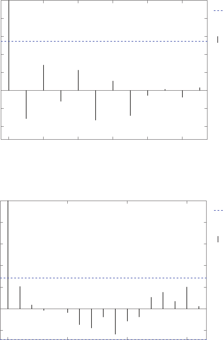
64 Flood-Frequency Estimation for Very Low Annual Exceedance Probabilities
0 2 4 6 8 10
−0.4
−0.2
0
0.2
0.4
0.6
0.8
1.0
Lag, in water years (all peaks treated as consecutive)
Autocorrelation
Line of statistical significance—
Autocorrelations that cross
these lines are statistically
significant at a 0.05
significance level
Autocorrelation
EXPLANATION
Station 09337500, Escalante River near Escalante, Utah
Figure 50. The autocorrelation for peaks in systematic period of record for streamgage station 09337500, Escalante River near
Escalante, Utah, 1943–55.
0 5 10 15
−0.2
0
0.2
0.4
0.6
0.8
1.0
Lag, in water years (all peaks treated as consecutive)
Autocorrelation
Line of statistical significance—
Autocorrelations that cross
these lines are statistically
significant at a 0.05
significance level
Autocorrelation
EXPLANATION
Station 09337500, Escalante River near Escalante, Utah
Figure 51. The autocorrelation for peaks in systematic period of record for streamgage station 09337500, Escalante River near
Escalante, Utah, 1972–2015.

Case Study Results and Discussion 65
EXPLANATION
●
Observation (all peaks treated as consecutive)
Annual peak streamflow, in cubic feet per second
0 2 4 6 8 10 12 14
10
100
1,000
10,000
●
●
●
●
●
●
●
●
●
●
●
●
●
Station 09337500, Escalante River near Escalante, Utah
Mean of distribution of
annual peak streamflow
Annual peak streamflow
Figure 52. Change points in mean and variance for peaks in systematic period of record for streamgage station 09337500,
Escalante River near Escalante, Utah, 1943–55.
EXPLANATION
●
Observation (all peaks treated as consecutive)
Annual peak streamflow, in cubic feet per second
0 10 20 30 40 50
10
100
1,000
10,000
●
●
●
●
●
●
●
●
●
●
●
●
●
●
●
●
●
●
●
●
●
●
●
●
●
●
●
●
●
●
●
●
●
●
● ●
●
●
●
●
●
●
●
●
●
●
●
Station 09337500, Escalante River near Escalante, Utah
Mean of distribution of
annual peak streamflow
Annual peak streamflow
Figure 53. Change points in mean and variance for peaks in systematic period of record for streamgage station 09337500,
Escalante River near Escalante, Utah, 1972–2015.

66 Flood-Frequency Estimation for Very Low Annual Exceedance Probabilities
EXPLANATION
Mann-Kendall trend line for
systematic record and
historical peaks,
p-value=0.45
Mann-Kendall trend line for
systematic record,
p-value=0.72
●
1900 1920 1940 1960 1980 2000 2020
Annual peak streamflow, in cubic feet per second
10
20
50
100
200
500
1,000
2,000
5,000
10,000
Water year
●
●
●
●
●
●
●
●
●
●
●
●
●
●
●
●
●
●
●
●
●
●
●
●
●
●
●
●
●
●
●
●
●
●
●
●
●
●
●
●
●
●
●
●
●
●
●
●●
●
●
●
●
●
●
●
●
●
●
●
Station 09337500, Escalante River near Escalante, Utah
Trend lines
Annual peak streamflow
Historical peak
Figure 54. Mann Kendall test for trend in the peak-streamflow record for streamgage station 09337500, Escalante River near
Escalante, Utah.
EXPLANATION
Perception threshold, in
cubic feet per second
0 to infinity
17,700 to infinity
Censored flow
Interval flow
Gaged peak
Historical or paleoflood
peak
1920 1940 1960 1980 2000
Water year
0
10,000
20,000
30,000
40,000
Annual peak streamflow, in cubic feet per second
Station 09337500, Escalante River near Escalante, Utah
Figure 55. Peaks and thresholds for flood-frequency analysis, Escalante River near Escalante, Utah.

Case Study Results and Discussion 67
Annual peak streamflow, in cubic feet per second
EXPLANATION
Fitted frequency
Potentially influential low flood
(PILF) threshold
Confidence limit—5-percent lower,
95-percent upper
Gaged peak
PILF
0.00010.0010.010.10.5
2102550
70
909899.5
Annual exceedance probability, in percent
1
10
100
1,000
10,000
100,000
Peakfq v 7.2 run 10/6/2019 1:44:33 PM
Expected Moments Algorithm (EMA) using
Weighted Skew option
−0.433 = Skew (G)
Multiple Grubbs-Beck
0 Zeroes not displayed
0 Censored flows below PILF (LO) Threshold
9 Gaged peaks below PILF (LO) Threshold
Station 09337500, Escalante River near Escalante, Utah
Figure 56. Annual exceedance probabilities for streamgage station 09337500, Escalante River near Escalante, Utah, using the
systematic peaks only (scenario 1).
Annual exceedance probability, in percent
Annual peak streamflow, in cubic feet per second
EXPLANATION
Fitted frequency
Potentially influential low flood
(PILF) threshold
Confidence limit—5-percent lower,
95-percent upper
Gaged peak
PILF
Historical peak
0.00010.010.10.5
2102550
70
909899.5
1
10
100
1,000
10,000
100,000
1,000,000
Peakfq v 7.2 run 12/6/2019 3:43:57 PM
Expected Moments Algorithm (EMA) using
Weighted Skew option
−0.384 = Skew (G)
Multiple Grubbs-Beck
0 Zeroes not displayed
0 Censored flows below PILF (LO) Threshold
9 Gaged peaks below PILF (LO) Threshold
Station 09337500, Escalante River near Escalante, Utah
Figure 57. Annual exceedance probabilities for streamgage station 09337500, Escalante River near Escalante, Utah, using the input
data depicted in figure 55.

68 Flood-Frequency Estimation for Very Low Annual Exceedance Probabilities
and the large paleoood peaks. It is possible the large paleo-
ood peaks are the result of unique climatic conditions. The
ood-frequency analyses of Webb and others (1988) and Webb
and Rathburn (1988), completed when the gage record was
substantially shorter, show these peaks as standing out from
the rest. However, in this study, the paleoood point estimates
fall within the error bounds of the tted frequency curve and,
therefore, magnitudes for very low AEPs were estimated.
Inclusion of the large paleoood peaks dramatically increases
the condence limits for the very low AEPs.
The AEPs calculated under these dierent scenarios
are compared graphically in gures 59–64. Figure 60 also
includes point estimates of magnitudes calculated for an AEP
of 0.01 in other studies discussed in the next section.
Comparisons to Other Flood-Frequency Methods
Kenney and others (2008) estimated ood frequencies
for the Escalante River site using the streamgage data through
water year 2005 and the three historical peaks. Their AEP of
0.01 estimate is provided in table 8. The dataset and methodol-
ogy are comparable to scenario 2 in this study, and their esti-
mate was 5,290 ft
3
/s, whereas the estimate in the current study
with 10 additional years of gaged record was 4,794 ft
3
/s.
Webb and others (1988) used gaged data through 1985;
gaged data plus 4 paleoood peaks; and gaged data, 4 paleo-
ood peaks, and a threshold indicating that the paleoood
peaks were the largest since 1875. The scenarios using the
data from Webb and others (1988) were designated as scenar-
ios 5–7 in gure 60 and table 8. Scenario 5 is like scenario 1
and falls within the condence bounds for the estimate at AEP
of 0.01. It is, however, higher than the estimate in scenario 1,
and this shows how the much longer gaged record in sce-
nario 1 reduced the ood magnitude estimate. Scenario 7 is
very similar to scenario 3 with slightly dierent assumptions
about the appropriate starting period (1909 for scenario 3 and
1875 for scenario 7). The estimates are similar: 15,730 ft
3
/s
for scenario 3, with the shorter beginning threshold and longer
gaging period, and 17,000 ft
3
/s for scenario 7.
Scenario 8 includes nine additional paleoood peaks
described by Webb and Rathburn (1988) as “prehistoric”
peaks. They reference Webb and others (1988) for these peaks,
but the nine “prehistoric” peaks are not quantied or used in
ood-frequency analysis there; however, dates were estimated
with considerable uncertainty for oods from approximately
A.D. 450 to A.D. 1550. The dates for large oods had uncer-
tainties as much as plus or minus 110 years in strata that had
date uncertainties as much as plus or minus 860 years (Webb
and others, 1988). Webb and Rathburn (1988) graphically
depict these nine oods indicating they had determined inter-
val estimates and selected years for plotting, but those values
are not listed. The graphical depiction hints that the Escalante
River analysis could be extended even further back in time,
but that was not done here because of the date and magnitude
uncertainties, as well as indications of signicant channel
change (Webb and others, 1988). Scenario 8’s estimate of
EXPLANATION
0.00010.010.10.5
2102550
70
909899.5
Annual exceedance probability, in percent
10
100
1,000
10,000
100,000
1,000,000
10,000,000
100,000,000
Annual peak streamflow, in cubic feet per second
Peakfq v 7.2 run 10/6/2019 1:51:22 PM
Expected Moments Algorithm (EMA) using
Weighted Skew option
0.225 = Skew (G)
Multiple Grubbs-Beck
0 Zeroes not displayed
0 Censored flows below PILF (LO) Threshold
9 Gaged peaks below PILF (LO) Threshold
Fitted frequency
Potentially influential low flood
(PILF) threshold
Confidence limit—5-percent lower,
95-percent upper
Censored flow
Interval flood estimate
Gaged peak
PILF
Historical or paleoflood peak
Station 09337500, Escalante River near Escalante, Utah
Figure 58. Annual exceedance probabilities for streamgage station 09337500, Escalante River near Escalante, Utah, using
systematic, historical, and paleoflood peaks and thresholds.

Case Study Results and Discussion 69
[Annual exceedance probability = 0.10]
PeakFQ 95-percent confidence interval
Mean of all point estimates,
3,027 cubic feet per second
PeakFQ point estimate
●
EXPLANATION
Streamflow, in cubic feet per second
0
2,000 4,000 6,000 8,000
Scenario 1
Scenario 2
Scenario 3
●
●
●
Station 09337500, Escalante River near Escalante, Utah
Figure 59. Point estimates and confidence bounds for streamgage station 09337500, Escalante River near Escalante, Utah, floods
with annual exceedance probability of 0.10, calculated under three different scenarios using U.S. Geological Survey PeakFQ software
(Veilleux and others, 2014) version 7.2. See table 8 for descriptions of the scenarios and the numeric values.
PeakFQ 95-percent confidence interval
[Annual exceedance probability = 0.01]
Mean of all point estimates,
11,237 cubic feet per second
PeakFQ point estimate
●
EXPLANATION
Streamflow, in cubic feet per second
0 10,000 20,000 30,000 40,000
Scenario 1
Scenario 2
Scenario 3
Scenario 4
Scenario 5
Scenario 6
Scenario 7
Scenario 8
Peak estimate from Kenney and others (2008)
Peak estimate from Webb and others (1988)
Peak estimate from Webb and Rathburn (1988)
●
●
●
Station 09337500, Escalante River near Escalante, Utah
Figure 60. Point estimates and confidence bounds for streamgage station 09337500, Escalante River near Escalante, Utah, floods
with annual exceedance probability of 0.01, calculated under three different scenarios using U.S. Geological Survey PeakFQ software
(Veilleux and others, 2014) version 7.2 compared to five point estimates from other studies (Kenney and others, 2008; Webb and others,
1988; Webb and Rathburn, 1988). See table 8 for descriptions of the scenarios and the numeric values.
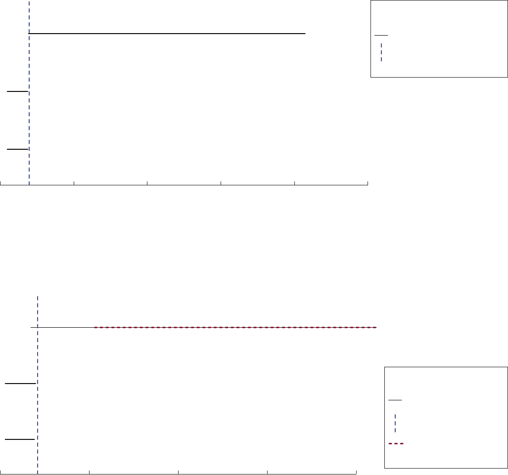
70 Flood-Frequency Estimation for Very Low Annual Exceedance Probabilities
PeakFQ 95-percent confidence interval
[Annual exceedance probability = 1×10
−3
]
Mean of all point estimates,
19,645 cubic feet per second
PeakFQ point estimate
●
EXPLANATION
Streamflow, in cubic feet per second
0
50,000 100,000 150,000 200,000 250,000
Scenario 1
Scenario 2
Scenario 3
●
●
●
Station 09337500, Escalante River near Escalante, Utah
Figure 61. Point estimates and confidence bounds for streamgage station 09337500, Escalante River near Escalante, Utah, floods with
annual exceedance probability of 1×10
−3
, calculated under three different scenarios using U.S. Geological Survey PeakFQ software
(Veilleux and others, 2014) version 7.2. See table 8 for descriptions of the scenarios and the numeric values.
Upper bound extends beyond
x-axis scale
PeakFQ 95-percent confidence
interval
[Annual exceedance probability = 1×10
−4
]
Mean of all point estimates,
42,263 cubic feet per second
PeakFQ point estimate
●
EXPLANATION
Streamflow, in cubic feet per second
0
100,000 200,000 300,000 400,000
Scenario 1
Scenario 2
Scenario 3
Upper bound is 1,136,000 cubic feet
per second
●
●
●
Station 09337500, Escalante River near Escalante, Utah
Figure 62. Point estimates and confidence bounds for streamgage station 09337500, Escalante River near Escalante, Utah, floods with
annual exceedance probability of 1×10
−4
, calculated under three different scenarios using U.S. Geological Survey PeakFQ software
(Veilleux and others, 2014) version 7.2. See table 8 for descriptions of the scenarios and the numeric values.

Case Study Results and Discussion 71
Upper bound extends beyond
x-axis scale
PeakFQ 95-percent confidence
interval
[Annual exceedance probability = 1×10
−5
]
Mean of all point estimates,
87,147 cubic feet per second
PeakFQ point estimate
●
EXPLANATION
Streamflow, in cubic feet per second
0
100,000 200,000 300,000 400,000 500,000
Scenario 1
Scenario 2
Scenario 3
Upper bound is 6,139,000 cubic feet
per second
●
●
●
Station 09337500, Escalante River near Escalante, Utah
Figure 63. Point estimates and confidence bounds for streamgage station 09337500, Escalante River near Escalante, Utah, floods with
annual exceedance probability of 1×10
−5
, calculated under three different scenarios using U.S. Geological Survey PeakFQ software
(Veilleux and others, 2014) version 7.2. See table 8 for descriptions of the scenarios and the numeric values.
Upper bound extends beyond
x-axis scale
PeakFQ 95-percent confidence
interval
[Annual exceedance probability = 1×10
−6
]
Mean of all point estimates,
173,603 cubic feet per second
PeakFQ point estimate
●
EXPLANATION
Streamflow, in cubic feet per second
0
200,000 400,000 600,000 800,000 1,000,000
Scenario 1
Scenario 2
Scenario 3
Upper bound is 32,790,000 cubic feet
per second
●
●
●
Station 09337500, Escalante River near Escalante, Utah
Figure 64. Point estimates and confidence bounds for streamgage station 09337500, Escalante River near Escalante, Utah, floods with
annual exceedance probability of 1×10
−6
, calculated under three different scenarios using U.S. Geological Survey PeakFQ software
(Veilleux and others, 2014) version 7.2. See table 8 for descriptions of the scenarios and the numeric values.
72 Flood-Frequency Estimation for Very Low Annual Exceedance Probabilities
an AEP of 0.01 is 13,100 ft
3
/s indicating that the addition of
paleoood information going back to A.D. 450 reduced the
peak estimate. This estimate is within the condence bounds
for scenario 3 (table 8 and g. 60).
Summary
The Escalante River had no autocorrelation, no change
points, and no trend. This site would seem to be a suitable can-
didate for extending the record with paleoood peaks to rene
condence limits for very low AEPs. AEPs calculated under
the three PeakFQ scenarios are summarized in gures 65 and
66. The gures show that adding paleoood information does
not always decrease uncertainty. The paleoood peaks added
were very large peaks and increased the uncertainty for very
low AEPs, while also increasing the estimated magnitudes.
The eect of the addition of paleoood peaks at this site is
similar to the eect at Spring Creek where the paleoood
peaks and single systematic outlier formed their own group
at much larger magnitudes than the systematic record. The
regional transfer experiment at Spring Creek showed that
if the space between the two distributions could be lled in
with additional peaks, the t might improve. Going back
much further in time, Webb and Rathburn (1988) added more
paleoood data to their ood-frequency analysis and reduced
the estimate for an AEP of 0.01. However, their condence
bounds are unknown, and their exact data were unable to be
replicated for this study. To further understand very low AEPs
at this site, more study would need to be done on persistent
climatic conditions and channel changes over time.

Case Study Results and Discussion 73
[Systematic data]
PeakFQ 95-percent confidence
interval
PeakFQ point estimate
●
EXPLANATION
[Systematic data]
PeakFQ 95-percent confidence
interval
PeakFQ point estimate
●
EXPLANATION
A
B
Streamflow, in cubic feet per second
0 20,000 40,000 60,000 80,000
2,486 cubic feet per second, annual exceedance probability = 0.10
4,962 cubic feet per second, annual exceedance probability = 0.01
7,622 cubic feet per second, annual exceedance probability = 1×10
−3
10,370 cubic feet per second, annual exceedance probability = 1×10
−4
13,140 cubic feet per second, annual exceedance probability = 1×10
−5
15,870 cubic feet per second, annual exceedance probability = 1×10
−6
Streamflow, in cubic feet per second
0 50,000 100,000 150,000 200,000
2,388 cubic feet per second, annual exceedance probability = 0.10
4,794 cubic feet per second, annual exceedance probability = 0.01
7,464 cubic feet per second, annual exceedance probability = 1×10
−3
10,320 cubic feet per second, annual exceedance probability = 1×10
−4
13,300 cubic feet per second, annual exceedance probability = 1×10
−5
16,340 cubic feet per second, annual exceedance probability = 1×10
−6
●
●
●
●
●
●
●
●
●
●
●
●
Station 09337500, Escalante River near Escalante, Utah
Figure 65. Point and interval estimates for a range of annual exceedance probabilities for streamgage station 09337500, Escalante
River near Escalante, Utah, floods, calculated using U.S. Geological Survey PeakFQ version 7.2, with A, as weighted skew and
systematic data and B, as weighted skew systematic plus historical data. This depicts analysis results for A, scenario 1 and B, scenario
2 of table 8.

74 Flood-Frequency Estimation for Very Low Annual Exceedance Probabilities
Summary
Very low probability oods may have an annual exceed-
ance probability (AEP) less than 0.001, meaning the mean
recurrence interval may be more than 1,000 years. Yet, estima-
tion of these ood frequencies is needed to accurately portray
risks to critical infrastructure, such as nuclear powerplants
and large dams. Standard methods for statistical estimation
of ood frequency rely on the systematic streamow record,
which provides a time series of annual maximum ood peaks.
Uncertainties are large when trying to extrapolate magnitudes
of very low AEP events from a streamow record that is much
shorter (typically less than 100 years). An additional complica-
tion for ood-frequency analysis is the underlying assumption
that the ood series is stationary. That is, the peak-ow time
series varies around a constant mean within a particular range
of values (a dened variance). As the hydrologic community’s
understanding of natural systems and anthropogenic eects
has evolved, it has become clear that the stationarity assump-
tion is sometimes inappropriate. However, there is not a con-
sensus on the appropriate methodology for the computation of
ood frequencies for nonstationary systems.
Flood-frequency analysis under nonstationary conditions
is an active area of research, and many suggested methods
are not yet able to incorporate paleoood data. However, a
literature review was completed to summarize the state of
ood-frequency science. The literature review highlights tools
available to detect nonstationarities and identify possible
attributing factors, and highlights eorts to include external
information for detection of nonstationarities. Additionally, the
review contributes to the understanding of underlying causes
of nonstationarities and potential ways to address nonstation-
arities, while simultaneously showing that the problem is not
easy to address.
Five sites were selected to demonstrate methods for ini-
tial data analysis and detection of trends and for incorporation
of historical and paleoood information in ood-frequency
analysis. The ood-frequency results should not be considered
denitive at any of these sites. The purpose of this analysis
was to study the eect of historical and paleoood data on the
ood-frequency distribution. Some subjectivity is inherent in
assessing the validity of historical and paleoood data and in
incorporating thresholds for missing periods during the sys-
tematic record and for paleo periods. Local or regional experts
might make dierent choices when assessing these sites.
The sites were Red River of the North at James Avenue
Pumping Station, Winnipeg, Manitoba, Canada (Red River);
lower reach, Rapid Creek, South Dakota (lower reach, Rapid
Creek); Spring Creek, South Dakota (Spring Creek); Cherry
Creek near Melvin, Colorado (Cherry Creek); and Escalante
River near Escalante, Utah (Escalante River). The sites were
chosen for geographic diversity and their unique characteris-
tics, which highlighted issues such as autocorrelation, outlier
peaks, or short period of record.
Streamflow, in cubic feet per second
0 200,000 400,000 600,000 800,000 1,000,000
4,206 cubic feet per second, annual exceedance probability = 0.10
15,730 cubic feet per second, annual exceedance probability = 0.01
43,850 cubic feet per second, annual exceedance probability = 1×10
−3
106,100 cubic feet per second, annual exceedance probability = 1×10
−4
235,000 cubic feet per second, annual exceedance probability = 1×10
−5
488,600 cubic feet per second, annual exceedance probability = 1×10
−6
Upper bound is 359,600,000 cubic feet
per second
Upper bound is 6,139,000 cubic feet
per second
Upper bound is 32,790,000 cubic feet
per second
●
●
●
●
●
●
[Systematic and paleoflood
data, weighted skew]
PeakFQ 95-percent confidence
interval
Upper bound extends beyond
x-axis scale
PeakFQ point estimate
●
EXPLANATION
Station 09337500, Escalante River near Escalante, Utah
Figure 66. Point and interval estimates for a range of annual exceedance probabilities for streamgage station 09337500, Escalante
River near Escalante, Utah, floods, calculated using U.S. Geological Survey PeakFQ version 7.2, with weighted skew and systematic,
historical, and paleoflood data. This depicts analysis results for scenario 3 of table 8.
Summary 75
The peaks for these sites were all analyzed for indica-
tors of nonstationarity including autocorrelation, change
points, and monotonic trends. Detected nonstationarities can
be naturally occurring, anthropogenically induced, or can
be statistical artifacts in the data. Therefore, it is dicult to
say when a nonstationarity disqualies a site or a period for
ood-frequency analysis, and the degree to which one of these
issues will aect ood frequency is dicult to assess.
The ood-frequency analysis completed for this study
used version 7.2 of the U.S. Geological Survey PeakFQ
program with extended output for AEPs as low as 1×10
−6
.
PeakFQ assumes that the peak-ow series follow a log-
Pearson type III distribution. This distribution is widely
used in hydrology, particularly in the United States, where
it is used in Bulletin 17C, which provides guidelines used
by some Federal agencies in the determination of ood ow
frequencies (under specic recommended assumptions).
Applications of the distribution use systematically collected
and historical peak-streamow values to dene a frequency
distribution based on the sample mean (location), standard
deviation (scale), and skew (shape). This study estimates those
distribution parameters using the expected moments algo-
rithm. Nonstandard ood data may be used with the expected
moments algorithm, including ood interval estimates, as
opposed to the standard point estimates and ood thresholds.
When other ood-frequency studies were available, their
results were compared to the results here. The comparisons in
some cases simply show the eect of additional years of data,
whereas other comparisons show results from methods other
than PeakFQ that use dierent probability distributions or t-
ting methods.
The Red River was chosen because of the availability of
well documented historical peaks and paleoood peaks. The
site has autocorrelated peaks; among the implications for this
is that 117 peaks on the Red River may have equivalent infor-
mation to 45 independent peaks. The Red River had a change
point in mean and variance. The change point and autocorrela-
tion are related to well documented climatic persistence in this
basin. The Red River also has an increasing peak magnitude
trend, likely more than just an artifact of climatic persis-
tence at the end of the record. Flood-frequency analysis was
completed under 11 dierent scenarios to show how regional
information, in the form of a weighted skew, and incremen-
tally adding data of dierent types (historical peaks, historical
intervals, paleoood data, and thresholds) aects the ood-
frequency analysis. In addition, several other ood-frequency
studies were compared so that for an AEP of 0.01, 23 dierent
scenarios were compared numerically and graphically. The
addition of peaks and thresholds beyond the systematic record
can increase the precision and accuracy of estimates for very
low AEPs (less than 0.001); in fact, paleoood data appear
necessary to reduce uncertainty for very low AEPs at this site.
When compared to another study that adjusted for correla-
tion, the addition of paleoood data, creating a much longer
record, appears to oset the loss of information caused by
correlated data.
The lower reach of Rapid Creek, chosen because of the
existence of paleoood data in a well-documented study, did
not have autocorrelation but did have one high outlier peak
that aects the t of the upper end of the distribution when
calculating ood frequencies. Paleoood information helped
put the outlier in context; however, very low AEPs at this site
still had extraordinarily large condence bounds.
Spring Creek, chosen because of the existence of paleo-
ood data in a well-documented study and because it was
nearby the lower reach of Rapid Creek for an experiment in
information transfer, was like the lower reach of Rapid Creek
in that it was uncorrelated and had a single outlier. This site
showed that peaks outside the systematic period of record
need to be examined carefully to determine whether they are
opportunistic peaks, which do not provide additional infor-
mation about appropriate thresholds for missing periods, or
whether they are large peaks from which a threshold can be
derived. Although generally helpful in determining very low
AEPs, paleoood data can increase uncertainty or worsen
the t of the upper end of the distribution if they appear to
come from a dierent, larger, population than the peaks in
the systematic record. Ideally, the range of paleoood peaks
should have some overlap with the observed range to provide
a smooth transition of the distribution. This site was also
used as an experiment in transferring regional paleoood
data—transferring information from the lower reach of Rapid
Creek to this site. This transfer of information provided more
information for the upper end of the distribution. However, the
transfer was based on methods that need more development
and renement for future applications.
Cherry Creek was used to compare the results with
paleoood data to results for distributions described in Asquith
and others (2017). This showed that the generalized Pareto
distribution was not a good distribution for estimating very
low AEPs, as Asquith and others (2017) found. The asymmet-
ric exponential power distribution and the generalized logistic
distribution generated large estimates for very low AEPs and
were not good distributions for this site. Of the remaining dis-
tributions, it appears that the best may depend on which AEP
is desired. In an analysis that is not exploratory, how to weight
the quantiles at given AEPs for the acceptable distributions
would need to be determined by subject matter experts.
The Escalante River was chosen because of the existence
of paleoood data and past ood-frequency analyses using
these data. Peaks at this site did not have autocorrelation,
change points, or a monotonic trend. This river has been the
subject of several paleoood studies and some of the paleo-
ood data were incorporated here. The paleoood peaks added
were very large peaks and increased the uncertainty for very
low AEPs.
The addition of historical peaks, paleoood peaks and
paleoood thresholds can increase or decrease the magnitude
of very low AEP oods, depending on the distribution and
length of the systematic period. The additional information can
reduce the error bounds on oods with very low exceedance
probabilities; however, the eect is not uniform across sites.
76 Flood-Frequency Estimation for Very Low Annual Exceedance Probabilities
References Cited
Abramowitz, M., and Stegun, I.A., eds., 1965, Handbook of
mathematical functions with formulas, graphs and math-
ematical tables: Dover, N.Y., 1046 p.
Acreman, M.C., and Wiltshire, S.E., 1987, Identication
of regions for regional ood frequency analysis: Eos
(Washington, D.C.), v. 68, no. 44.
Allaby, M., ed., 2008, A dictionary of earth sci-
ences (3d ed.): Oxford University Press, Oxford,
United Kingdom, accessed August 4, 2018, at
https://www.oxfordreference.com/ view/ 10.1093/ acref/
9780199211944.001.0001/ acref- 9780199211944.
Armstrong, W.H., Collins, M.J., and Snyder, N.P., 2012,
Increased frequency of low-magnitude oods in New
England: Journal of the American Water Resources
Association, v. 48, no. 2, p. 306–320. [Also available at
https://doi.org/ 10.1111/ j.1752- 1688.2011.00613.x.]
Asquith, W.H., 2001, Eects of regulation on L-moments
of annual peak streamow in Texas: U.S. Geological
Survey Water-Resources Investigations Report 01–4243,
66 p., accessed July 23, 2018, at https://doi.org/ 10.3133/
wri014243.
Asquith, W.H., 2011, Distributional analysis with L-moment
statistics using the R environment for statistical comput-
ing: Lubbock, Tex., Create Space Independent Publishing
Platform, 360 p.
Asquith, W.H., 2017, lmomco—L-moments, censored
L-moments, trimmed L-moments, L-comoments, and
many distributions: R package version 2.2.9., accessed
February 28, 2017, at https://cran.r- project.org/ web/
packages/ lmomco/ index.html.
Asquith, W.H., Kiang, J.E., and Cohn, T.A., 2017, Application
of at-site peak-streamow frequency analyses for very low
annual exceedance probabilities: U.S. Geological Survey
Scientic Investigations Report 2017–5038, 93 p. [Also
available at https://doi.org/ 10.3133/ sir20175038.]
Auger, I.E., and Lawrence, C.E., 1989, Algorithms for the
optimal identication of segment neighborhoods: Bulletin
of Mathematical Biology, v. 51, no. 1, p. 39–54. [Also avail-
able at https://doi.org/ 10.1016/ S0092- 8240(89)80047- 3.]
Ayalew, T.B., Krajewski, W.F., and Mantilla, R., 2013,
Exploring the eect of reservoir storage on peak discharge
frequency: Journal of Hydrologic Engineering, v. 18, no. 12,
p. 1697–1708. [Also available at https://doi.org/ 10.1061/
(ASCE)HE.1943- 5584.0000721.]
Ayalew, T.B., Krajewski, W.F., Mantilla, R., Wright, D.B., and
Small, S.J., 2017, Eect of spatially distributed small dams
on ood frequency—Insights from the Soap Creek water-
shed: Journal of Hydrologic Engineering, v. 22, no. 7, 11 p.
[Also available at https://doi.org/ 10.1061/ (ASCE)HE.1943-
5584.0001513.]
Ballesteros Cánovas, J.A., Eguibar, M., Bodoque, J.M.,
Díez-Herrero, A., Stoel, M., and Gutiérrez-Pérez, I., 2011,
Estimating ash ood discharge in an ungauged mountain
catchment with 2D hydraulic models and dendrogeo-
morphic palaeostage indicators: Hydrological Processes,
v. 25, no. 6, p. 970–979. [Also available at https://doi.org/
10.1002/ hyp.7888.]
Ballesteros Cánovas, J.A., Trappmann, D., Shekhar, M.,
Bhattacharyya, A., and Stoel, M., 2017, Regional ood-
frequency reconstruction for Kullu district, Western Indian
Himalayas: Journal of Hydrology, v. 546, p. 140–149. [Also
available at https://doi.org/ 10.1016/ j.jhydrol.2016.12.059.]
Baranowski, R., and Fryzlewicz, P., 2015, wbs—Wild
binary segmentation for multiple change-point detection:
R package version 1.3, accessed February 28, 2017, at
https://CRAN.R- project.org/ package= wbs.
Barendregt, R.W., and Irving, E., 1998, Changes in the
extent of North American ice sheets during the late
Cenozoic: Canadian Journal of Earth Sciences, v. 35, no. 5,
p. 504–509. [Also available at https://doi.org/ 10.1139/
e97- 126.]
Barry, D., and Hartigan, J.A., 1993, A Bayesian analysis for
change point problems: Journal of the American Statistical
Association, v. 35, no. 3, p. 309–319.
Bartles, M., Brunner, G., Fleming, M., Faber, B., and
Slaughter, J., 2016, HEC-SSP—Statistical software pack-
age version 2.1: U.S. Army Corps of Engineers Computer
Program Documentation, 379 p., accessed August 4, 2018,
at https://www.hec.usace.army.mil/ software/ hec- ssp/
documentation/ HEC- SSP_ 21_ Users_ Manual.pdf.
Bayazit, M., 2015, Nonstationarity of hydrological records and
recent trends in trend analysis—A state-of-the-art review:
Environmental Processes, v. 2, no. 3, p. 527–542. [Also
available at https://doi.org/ 10.1007/ s40710- 015- 0081- 7.]
Bayazit, M., and Önöz, B., 2007, To prewhiten or not to pre-
whiten in trend analysis?: Hydrological Sciences Journal,
v. 52, no. 4, p. 611–624. [Also available at https://doi.org/
10.1623/ hysj.52.4.611.]
References Cited 77
Benito, G., Lang, M., Barriendos, M., Llasat, M.C., Francés,
F., Ouarda, T., Thorndycraft, V., Enzel, Y., Bardossy, A.,
Coeur, D., and Bobée, B., 2004, Use of systematic, palaeo-
ood and historical data for the improvement of ood risk
estimation—Review of scientic methods: Natural Hazards,
v. 31, no. 3, p. 623–643. [Also available at https://doi.org/
10.1023/ B:NHAZ.0000024895.48463.eb.]
Beran, J., 1994, Statistics for long-memory processes—
Monographs on statistics and applied probability: New
York, Chapman & Hall/CRC, 315 p.
Bluemle, J.P., 1996, From the state geologist: North Dakota
Geological Survey Newsletter, v. 23, no. 1, p. 1–2.
Booy, C., and Lye, L.M., 1989, A new look at ood risk
determination: Water Resources Bulletin, v. 25, no. 5,
p. 933–943. [Also available at https://doi.org/ 10.1111/
j.1752- 1688.1989.tb05407.x.]
Booy, C., and Morgan, D.R., 1985, The eect of cluster-
ing of ood peaks on a ood risk analysis for the Red
River: Canadian Journal of Civil Engineering, v. 12, no. 1,
p. 150–165. [Also available at https://doi.org/ 10.1139/
l85- 015.]
Brath, A., Castellarin, A., Franchini, M., and Galeati,
G., 2001, Estimating the index ood using indirect
methods: Hydrological Sciences Journal, v. 46, no. 3,
p. 399–418. [Also available at https://doi.org/ 10.1080/
02626660109492835.]
Bronaugh, D., and Werner, A., 2013, zyp: Zhang + Yue-
Pilon trends package: R package version 0.10-1, accessed
February 28, 2017, at https://CRAN.R- project.org/
package= zyp.
Buckley, J.J., and Jowers, L.J., 2008, Monte Carlo methods
in fuzzy optimization: Berlin, Springer-Verlag, Studies in
Fuzziness and Soft Computing, 260 p.
Burn, D.H., 1990a, An appraisal of the “region of inu-
ence” approach to ood frequency analysis: Hydrological
Sciences Journal, v. 35, no. 2, p. 149–165. [Also available at
https://doi.org/ 10.1080/ 02626669009492415.]
Burn, D.H., 1990b, Evaluation of regional ood frequency
analysis with a region of inuence approach: Water
Resources Research, v. 26, no. 10, p. 2257–2265. [Also
available at https://doi.org/ 10.1029/ WR026i010p02257.]
Burn, D.H., and Goel, N.K., 2001, Flood frequency analysis
for the Red River at Winnipeg: Canadian Journal of Civil
Engineering, v. 28, no. 3, p. 355–362. [Also available at
https://doi.org/ 10.1139/ l00- 122.]
Busuioc, A., and von Storch, H.V., 1996, Changes in the
winter precipitation in Romania and its relation to the large‐
scale circulation: Tellus. Series A, Dynamic Meterology and
Oceanography, v. 48, no. 4, p. 538–552. [Also available at
https://doi.org/ 10.1034/ j.1600- 0870.1996.t01- 3- 00004.x.]
Buttle, J.M., 2011, Streamow response to headwater
reforestation in the Ganaraska River basin, southern
Ontario, Canada: Hydrological Processes, v. 25, no. 19,
p. 3030–3041. [Also available at https://doi.org/ 10.1002/
hyp.8061.]
Caeiro, F., and Mateus, A., 2014, randtests—Testing random-
ness in R: R package version 1.0, accessed February 28,
2017, at https://CRAN.R- project.org/ package= randtests.
Canada Department of Resources and Development, 1953,
Report on investigations into measures for the reduction of
the ood hazard in the greater Winnipeg area: Red River
Basin Investigation, Water Resources Division, Engineering
and Water Resources Branch, 66 p., 8 appendices.
Carslaw, D.C., and Ropkins, K., 2012, openair—An R pack-
age for air quality data analysis: Environmental Modelling
& Software, v. 27–28, p. 52–61. [Also available at
https://doi.org/ 10.1016/ j.envsoft.2011.09.008.]
Castellarin, A., Vogel, R.M., and Matalas, N.C., 2005,
Probabilistic behavior of a regional envelope curve: Water
Resources Research, v. 41, no. 6, 13 p. [Also available at
https://doi.org/ 10.1029/ 2004WR003042.]
Chiew, F.H.S., and McMahon, T.A., 1993, Detection of trend
or change in annual ow of Australian rivers: International
Journal of Climatology, v. 13, no. 6, p. 643–653. [Also
available at https://doi.org/ 10.1002/ joc.3370130605.]
Chiew, F., and Siriwardena, L., 2005, TREND—User guide:
CRC for Catchment Hydrology, 23 p.
Cohn, T.A., England, J.F., Berenbrock, C.E., Mason, R.R.,
Stedinger, J.R., and Lamontagne, J.R., 2013, A generalized
Grubbs-Beck test statistic for detecting multiple potentially
inuential low outliers in ood series: Water Resources
Research, v. 49, no. 8, p. 5047–5058. [Also available at
https://doi.org/ 10.1002/ wrcr.20392.]
Cohn, T.A., Lane, W.L., and Baier, W.G., 1997, An algorithm
for computing moments-based ood quantile estimates
when historical ood information is available: Water
Resources Research, v. 33, no. 9, p. 2089–2096. [Also avail-
able at https://doi.org/ 10.1029/ 97WR01640.]
Cohn, T.A., Lane, W.L., and Stedinger, J.R., 2001, Condence
intervals for expected moments algorithm ood quan-
tile estimates: Water Resources Research, v. 37, no. 6,
p. 1695–1706. [Also available at https://doi.org/ 10.1029/
2001WR900016.]
78 Flood-Frequency Estimation for Very Low Annual Exceedance Probabilities
Cohn, T.A., and Lins, H.F., 2005, Nature’s style—Naturally
trendy: Geophysical Research Letters, v. 32, no. 23, 5 p.
[Also available at https://doi.org/ 10.1029/ 2005GL024476.]
Conover, W.J., 1999, Practical nonparametric statistics: New
York, John Wiley & Sons, Inc., 584 p.
Cox, D.R., and Stuart, A., 1955, Some quick sign tests for
trend in location and dispersion: Biometrika, v. 42, no. 1/2,
p. 80–95. [Also available at https://doi.org/ 10.2307/
2333424.]
Crippen, J.R., and Bue, C.D., 1977, Maximum oodows in
the conterminous United States: U.S. Geological Survey
Water Supply Paper 1887, 52 p., accessed February 3, 2017,
at https://pubs.usgs.gov/ wsp/ 1887/ report.pdf.
Curran, J.H., Barth, N.A., Veilleux, A.G., and Ourso, R.T.,
2016, Estimating ood magnitude and frequency at gaged
and ungaged sites on streams in Alaska and conterminous
basins in Canada, based on data through water year 2012:
Scientic Investigations Report 2016–5024, 58 p., accessed
March 1, 2017, at https://pubs.er.usgs.gov/ publication/
sir20165024.
Dalrymple, T., 1960, Flood-frequency analyses, manual of
hydrology—Part 3: U.S. Geological Survey 1543–A, 80
p., accessed February 3, 2017, at https://pubs.er.usgs.gov/
publication/ wsp1543A.
Davison, A.C., and Hinkley, D.V., 1997, Bootstrap meth-
ods and their application—Cambridge series in statistical
and probabilistic mathematics: New York, Cambridge
University Press, 594 p. [Also available at https://doi.org/
10.1017/ CBO9780511802843.]
Dawdy, D.R., Gris, V.W., and Gupta, V.K., 2012, Regional
ood-frequency analysis—How we got here and where we
are going: Journal of Hydrologic Engineering, v. 17, no. 9,
p. 953–959. [Also available at https://doi.org/ 10.1061/
(ASCE)HE.1943- 5584.0000584.]
Dinicola, K., 1996, The “100-year ood”: U.S. Geological
Survey Fact Sheet 229-96, accessed February 28, 2017, at
https://pubs.usgs.gov/ fs/ FS- 229- 96/ pdf/ FS_ 229- 96.pdf.
Douglas, E.M., Vogel, R.M., and Kroll, C.N., 2000, Trends
in oods and low ows in the United States—Impact of
spatial correlation: Journal of Hydrology, v. 240, no. 1-2,
p. 90–105. [Also available at https://doi.org/ 10.1016/ S0022-
1694(00)00336- X.]
Dutta, D., Kim, S., Vaze, J., and Hughes, J., 2015,
Streamow predictions in regulated river systems—
Hydrological non-stationarity versus anthropogenic water
use: Proceedings of the International Association of
Hydrological Sciences, v. 371, p. 35–42. [Also available at
https://doi.org/ 10.5194/ piahs- 371- 35- 2015.]
Eng, K., Chen, Y.-Y., and Kiang, J.E., 2009, User’s guide to
the weighted-multiple-linear regression program (WREG
version 1.0): Techniques and Methods, book 4, chap. A8, 21
p., accessed September 2, 2018, at https://pubs.er.usgs.gov/
publication/ tm4A8.
Eng, K., Kiang, J.E., Chen, Y.-Y., Carlisle, D.M., and Granato,
G.E., 2011, Causes of systematic over- or underestimation
of low streamows by use of index-streamgage approaches
in the United States: Hydrological Processes, v. 25, no. 14,
p. 2211–2220. [Also available at https://doi.org/ 10.1002/
hyp.7976.]
Eng, K., Milly, P.C., and Tasker, G.D., 2007, Flood
Regionalization—A hybrid geographic and predictor-
variable region-of-inuence regression method: Journal
of Hydrologic Engineering, v. 12, no. 6, p. 585–591.
[Also available at https://doi.org/ 10.1061/ (ASCE)1084-
0699(2007)12:6(585).]
Eng, K., Tasker, G.D., and Milly, P.C.D., 2005, An analysis of
region-of-inuence methods for ood regionalization in the
Gulf-Atlantic Rolling Plains: Journal of the American Water
Resources Association, v. 41, no. 1, p. 135–143. [Also avail-
able at https://doi.org/ 10.1111/ j.1752- 1688.2005.tb03723.x.]
England, J.F., Jr.; Cohn, T.A.; Faber, B.A.; Stedinger, J.R.;
Thomas, W.O., Jr.; Veilleux, A.G.; Kiang, J.E.; and Mason,
R.R., Jr., 2019, Guidelines for determining ood ow fre-
quency—Bulletin 17C (ver. 1.1, May 2019): U.S. Geologi-
cal Survey Techniques and Methods, book 4, chap. B5,
148 p., accessed March 1, 2017, at https://doi.org/10.3133/
tm4B5.
Enzel, Y., Ely, L.L., House, P.K., Baker, V.R., and Webb,
R.H., 1993, Paleoood evidence for a natural upper bound
to ood magnitudes in the Colorado River Basin: Water
Resources Research, v. 29, no. 7, p. 2287–2297. [Also avail-
able at https://doi.org/ 10.1029/ 93WR00411.]
Erdman, C., and Emerson, J.W., 2007, bcp—An R package for
performing a Bayesian analysis of change point problems:
Journal of Statistical Software, v. 23, no. 3, p. 1–13. [Also
available at https://doi.org/ 10.18637/ jss.v023.i03.]
Eslamian, S., ed., 2014, Handbook of engineering
hydrology—Modeling climate change, and variability: New
York, CRC Press, 646 p. [Also available at https://doi.org/
10.1201/ b16683.]
Federal Emergency Management Agency, 2016, Why dams
fail: Federal Emergency Management Agency web page,
accessed February 28, 2017, at https://www.fema.gov/ why-
dams- fail.
References Cited 79
Filliben, J.J., and Heckert, A., 2012, Maximum likelihood,
in Croarkin, C., and Tobias, P., eds., NIST/SEMATECH
e-Handbook of Statistical Methods: Gaithersburg, Md.,
National Institute of Standards and Technology, accessed
January 24, 2017, at https://www.itl.nist.gov/ div898/
handbook/ eda/ section3/ eda3652.htm.
Flynn, K.M., Kirby, W.H., and Hummel, P.R., 2006, User’s
manual for program PeakFQ annual ood-frequency
analysis using Bulletin 17B guidelines: U.S. Geological
Survey, Techniques and Methods Book 4, Chapter B4, 42
p., accessed January 23, 2017, at https://pubs.usgs.gov/ tm/
2006/ tm4b4/ .
Freeman, W.B., and Leighton, M.O., 1911, Surface water
supply of the United States, 1909, Part IX, Colorado River
basin: Water Supply Paper 269, 247 p., accessed August 24,
2017, at https://pubs.er.usgs.gov/ publication/ wsp269.
Friedman, D., Schechter, J., Baker, B., Mueller, C.,
Villarini, G., and White, K.D., 2016, U.S. Army Corps of
Engineers nonstationarity detection tool user guide: U.S.
Army Corps of Engineers, accessed January 24, 2017,
at http://corpsmapu.usace.army.mil/ rccinfo/ nsd/ docs/
Nonstationarity_ Detection_ Tool_ User_ Guide.pdf.
Friedman, D., Schechter, J., Saint-Miller, A.M., Mueller, C.,
Villarini, G., White, K.D., and Baker, B., 2018, US Army
Corps of Engineers nonstationarity detection tool user
guide—Version 1.2—May 2016—User manual update—
September 2018: U.S. Army Corps of Engineers, accessed
April 22, 2018, at http://corpsmapu.usace.army.mil/ rccinfo/
nsd/ docs/ Nonstationarity_ Detection_ Tool_ User_ Guide.pdf.
Fryzlewicz, P., 2014, Wild binary segmentation for multiple
change-point detection: Annals of Statistics, v. 42, no. 6,
p. 2243–2281. [Also available at https://doi.org/ 10.1214/
14- AOS1245.]
Fuller, W.E., 1914, Flood ows, in Transactions of the
American society of civil engineers v. 77: New York,
American Society of Civil Engineers, p. 564–617.
Fulton, R.J., ed., 1989, Quaternary geology of Canada and
Greenland: Geological Survey of Canada, Geology of
Canada, no. 1, 839 p.
Gado T.A., and Nguyen, Van-Thanh-Van, 2016, Comparison
of homogeneous region delineation approaches for regional
ood frequency analysis at ungauged sites: Journal of
Hydrologic Engineering, v. 21, no. 3, p. 04015068 (1–10).
Gaume, E., Gaál, L., Viglione, A., Szolgay, J., Kohnová,
S., and Blöschl, G., 2010, Bayesian MCMC approach
to regional ood frequency analyses involving extraor-
dinary ood events at ungauged sites: Journal of
Hydrology, v. 394, no. 1–2, p. 101–117. [Also available at
https://doi.org/ 10.1016/ j.jhydrol.2010.01.008.]
Gilbert, R.O., 1987, Statistical methods for environmental
pollution monitoring: New York, Van Nostrand Reinhold
Co., 320 p.
Government of Canada, 2019, Real-time hydromet-
ric data graph for RED RIVER AT JAMES AVENUE
PUMPING STATION (05OJ015) [MB]: Government
of Canada database, accessed October 10, 2019, at
https://wateroce.ec.gc.ca/ report/ real_ time_ e.html?
stn= 05OJ015.
Grayson, R.B., Argent, R.M., Nathan, R.J., McMahon, T.A.,
and Mein, R.G., 1996, Hydrological recipes—Estimation
techniques in Australian hydrology: Australia, Cooperative
Research Centre for Catchment Hydrology, 125 p.
Greenbaum, N., Harden, T.M., Baker, V.R., Weisheit, J., Cline,
M.L., Porat, N., Halevi, R., and Dohrenwend, J., 2014, A
2000 year natural record of magnitudes and frequencies for
the largest Upper Colorado River oods near Moab, Utah:
Water Resources Research, v. 50, no. 6, p. 5249–5269.
[Also available at https://doi.org/ 10.1002/ 2013WR014835.]
Gris, V.W., and Stedinger, J.R., 2007, Evolution of ood
frequency analysis with Bulletin 17: Journal of Hydrologic
Engineering, v. 12, no. 3, p. 283–297. [Also available at
https://doi.org/ 10.1061/ (ASCE)1084- 0699(2007)12:3(283).]
Gris, V.W., Stedinger, J.R., and Cohn, T.A., 2004, Log
Pearson type 3 quantile estimators with regional skew
information and low outlier adjustments: Water Resources
Research, v. 40, no. 7, W07503. [Also available at
https://doi.org/ 10.1029/ 2003WR002697.]
Grover, P., Burn, D., and Cunderlik, J., 2002, A comparison
of index ood estimation procedures for ungauged catch-
ments: Canadian Journal of Civil Engineering, v. 29, no. 5,
p. 734–741. [Also available at https://doi.org/ 10.1139/
l02- 065.]
Haddad, K., and Rahman, A., 2012, Regional ood frequency
analysis in eastern Australia—Bayesian GLS regression-
based methods within xed region and ROI framework—
Quantile Regression vs. Parameter Regression Technique:
Journal of Hydrology, v. 430–431, p. 142–161. [Also avail-
able at https://doi.org/ 10.1016/ j.jhydrol.2012.02.012.]
Haddad, K., Rahman, A., and Ling, F., 2015, Regional ood
frequency analysis method for Tasmania, Australia—A
case study on the comparison of xed region and region-of-
inuence approaches: Hydrological Sciences Journal, v. 60,
no. 12, p. 2086–2101. [Also available at https://doi.org/
10.1080/ 02626667.2014.950583.]
Hamed, K.H., 2008, Trend detection in hydrologic data—The
Mann–Kendall trend test under the scaling hypothesis:
Journal of Hydrology, v. 349, no. 3-4, p. 350–363. [Also
available at https://doi.org/ 10.1016/ j.jhydrol.2007.11.009.]
80 Flood-Frequency Estimation for Very Low Annual Exceedance Probabilities
Hamed, K.H., and Rao, A.R., 1998, A modied Mann-
Kendall trend test for autocorrelated data: Journal of
Hydrology, v. 204, no. 1–4, p. 182–196. [Also available at
https://doi.org/ 10.1016/ S0022- 1694(97)00125- X.]
Harden, N., 1999, Red River ood frequency and risk analysis,
in Red River Flooding—Decreasing our Risks, Winnipeg,
Manitoba, 1999, Proceedings: Winnipeg Manitoba,
Canadian Water Resources Association Conference, p.
IV1–IV18.
Harden, T.M., and O’Connor, J.E., 2017, Prehistoric oods
on the Tennessee River—Assessing the use of stratigraphic
records of past oods for improved ood-frequency
analysis: U.S. Geological Survey Scientic Investigations
Report 2017–5052, 15 p., accessed September 30, 2016, at
https://doi.org/ 10.3133/ sir20175052.
Harden, T.M., O’Connor, J.E., and Driscoll, D.G., 2015, Late
Holocene ood probabilities in the Black Hills, South
Dakota with emphasis on the Medieval Climate Anomaly:
Past Hydrological Extreme Events in a Changing Climate,
v. 130, p. 62–68.
Harden, T.M., O’Connor, J.E., Driscoll, D.G., and Stamm,
J.F., 2011, Flood-frequency analyses from paleoood
investigations for Spring, Rapid, Boxelder, and Elk Creeks,
Black Hills, western South Dakota: U.S. Geological
Survey Scientic Investigations Report 2011–5131, 136 p.,
accessed September 30, 2016, at https://pubs.usgs.gov/ sir/
2011/ 5131/ .
Hazen, A., 1930, Flood ows—A study of frequencies and
magnitudes: New York, John Wiley & Sons, Inc., 199 p.
He, W., Wan, S., Jiang, Y., Jin, H., Zhang, W., Wu, Q., and
He, T., 2013, Detecting abrupt change on the basis of
skewness—Numerical tests and applications: Journal of
Climatology, v. 33, p. 2713–2727.
Helsel, D.R., and Hirsch, R.M., 1992, Statistical methods in
water resources: New York, Elsevier, 529 p.
Higgins, J.J., 2003, Introduction to modern nonparametric
statistics: Pacic Grove, California, Duxbury Press, 384 p.
Hirsch, R.M., 1982, A comparison of four streamow record
extension techniques: Water Resources Research, v. 18,
no. 4, p. 1081–1088. [Also available at https://doi.org/
10.1029/ WR018i004p01081.]
Hirsch, R.M., 2011, A perspective on nonstationarity and
water management: Journal of the American Water
Resources Association, v. 47, no. 3, p. 436–446. [Also avail-
able at https://doi.org/ 10.1111/ j.1752- 1688.2011.00539.x.]
Hirsch, R.M., and Ryberg, K.R., 2012, Has the magni-
tude of oods across the USA changed with global
CO2 levels?: Hydrological Sciences Journal, v. 57,
no. 1, p. 1–9. [Also available at https://doi.org/ 10.1080/
02626667.2011.621895.]
Hodgkins, G.A., and Dudley, R.W., 2011, Historical summer
base ow and stormow trends for New England rivers:
Water Resources Research, v. 47, no. 7, p. 1–16. [Also
available at https://doi.org/ 10.1029/ 2010WR009109.]
Hodgkins, G.A., Dudley, R.W., Archeld, S.A., and Renard,
B., 2019, Eects of climate, regulation, and urbanization
on historical ood trends in the United States: Journal
of Hydrology, v. 573, p. 697–709. [Also available at
https://doi.org/ 10.1016/ j.jhydrol.2019.03.102.]
Hodgkins, G.A., Whiteld, P.H., Burn, D.H., Hannaford, J.,
Renard, B., Stahl, K., Fleig, A.K., Madsen, H., Mediero, L.,
Korhonen, J., Murphy, C., and Wilson, D., 2017, Climate-
driven variability in the occurrence of major oods across
North America and Europe: Journal of Hydrology, v. 552,
p. 704–717. [Also available at https://doi.org/ 10.1016/
j.jhydrol.2017.07.027.]
Holmes, R.R., Jr., and Dinicola, K., 2010, 100-Year ood–
it’s all about chance: U.S. Geological Survey General
Information Product 106, 1 p. [Also available at
https://pubs.usgs.gov/ gip/ 106/ .]
Homer, C., Dewitz, J., Yang, L., Jin, S., Danielson, P.,
Xian, G., Coulston, J., Herold, N., Wickham, J., and
Megown, K., 2015, Completion of the 2011 National Land
Cover Database for the conterminous United States—
Representing a decade of land cover change information:
Photogrammetric Engineering and Remote Sensing, v. 81,
no. 0, p. 345–354.
Hosking, J.R.M., and Wallis, J.R., 1986, Paleoood hydrology
and ood frequency analysis: Water Resources Research,
v. 22, no. 4, p. 543–550. [Also available at https://doi.org/
10.1029/ WR022i004p00543.]
Hosking, J.R.M., and Wallis, J.R., 2005, Regional frequency
analysis—An approach based on L-moments: New York,
Cambridge University Press.
Hosman, K.J., Ely, L.L., and O’Connor, J.E., 2003, Holocene
paleoood hydrology of the lower Deschutes River, Oregon,
in O’Connor, J.E., and Grant, G.E., eds., A peculiar river—
Geology, geomorphology, and hydrology of the Deschutes
River, Oregon, (v. 7): American Geophysical Union, Water
Science and Application Series, p. 121–146.
Hurst, H.E., 1951, Long-term storage capacity of reservoirs:
Transactions of the American Society of Civil Engineers,
v. 116, no. 1, p. 770–799.
References Cited 81
Interagency Advisory Committee on Water Data, 1982,
Guidelines for determining ood ow frequency—Bulletin
17B of the hydrology subcommittee: U.S. Geological
Survey Interagency Advisory Committee on Water Data,
accessed February 21, 2017, at https://water.usgs.gov/ osw/
bulletin17b/ dl_ ow.pdf.
James, N.A., and Matteson, D.S., 2014, ecp—An R pack-
age for nonparametric multiple change point analysis of
multivariate data: Journal of Statistical Software, v. 62,
no. 7, p. 1–25. [Also available at https://doi.org/ 10.18637/
jss.v062.i07.]
Jarrett, R.D., 2000, Paleoood investigations for Cherry Creek
basin, eastern Colorado, in Joint Conference on Water
Resources Engineering and Water Resources Planning and
Management, Minneapolis, Minn., 2000, Proceedings:
Minneapolis, Minn., American Society of Civil Engineers,
p. 1–10. [Also available at https://doi.org/ 10.1061/
40517(2000)122.]
Jarrett, R.D., and Tomlinson, E.M., 2000, Regional interdisci-
plinary paleoood approach to assess extreme ood poten-
tial: Water Resources Research, v. 36, no. 10, p. 2957–2984.
[Also available at https://doi.org/ 10.1029/ 2000WR900098.]
Jarvis, C.S., 1936, Floods in the United States—Magnitude
and frequency: U.S. Geological Survey Water Supply
Paper 771, 495 p., accessed August 9, 2017, at
https://pubs.er.usgs.gov/ publication/ wsp771.
Javelle, P., Ouarda, T.B.M.J., Lang, M., Bobée, B., Galéa,
G., and Grésillon, J.-M., 2002, Development of regional
ood-duration–frequency curves based on the index-ood
method: Journal of Hydrology, v. 258, no. 1–4, p. 249–259.
[Also available at https://doi.org/ 10.1016/ S0022-
1694(01)00577- 7.]
Jin, M., and Stedinger, J.R., 1989, Flood frequency analysis
with regional and historical information: Water Resources
Research, v. 25, no. 5, p. 925–936. [Also available at
https://doi.org/ 10.1029/ WR025i005p00925.]
Kendall, M.G., 1938, A new measure of rank correlation:
Biometrika, v. 30, no. 1–2, p. 81–93. [Also available at
https://doi.org/ 10.1093/ biomet/ 30.1- 2.81.]
Kennedy, J.R., Paretti, N.V., and Veilleux, A.G., 2014,
Methods for estimating magnitude and frequency of 1-,
3-, 7-, 15-, and 30-day ood-duration ows in Arizona:
U.S. Geological Survey Scientic Investigations
Report 2014–5109, 45 p., accessed August 9, 2017, at
https://pubs.er.usgs.gov/ publication/ sir20145109.
Kenney, T.A., Wilkowske, C.D., and Wright, S.J., 2008,
Methods for estimating magnitude and frequency of peak
ows for natural streams in Utah: U.S. Geological Survey
Scientic Investigations Report 2007–5158, 28 p.
Khaliq, M.N., Ouarda, T.B.M.J., and Gachon, P., 2009,
Identication of temporal trends in annual and seasonal low
ows occurring in Canadian rivers—The eect of short-
and long-term persistence: Journal of Hydrology, v. 369,
no. 1–2, p. 183–197. [Also available at https://doi.org/
10.1016/ j.jhydrol.2009.02.045.]
Killick, R., and Eckley, I.A., 2014, changepoint—An R
package for changepoint analysis: Journal of Statistical
Software, v. 1, no. 3, p. 1–19.
Killick, R., Fearnhead, P., and Eckley, I.A., 2012a, Optimal
detection of changepoints with a linear computational cost:
Journal of the American Statistical Association, v. 107,
no. 500, p. 1590–1598. [Also available at https://doi.org/
10.1080/ 01621459.2012.737745.]
Killick, R., Fearnhead, P., and Eckley, I.A., 2016,
changepoint—An R package for changepoint analysis:
R package version 2.2.1, accessed September 30, 2016,
http://CRAN.R- project.org/ package= changepoint.
Killick, R., Nam, C.F.H., Aston, J.A.D., and Eckley, I.A.,
2012b, The changepoint repository: accessed February 1,
2017, at [Also available at http://changepoint.info.]
Kjeldsen, T.R., and Rosbjerg, D., 2002, Comparison of
regional index ood estimation procedures based on the
extreme value type I distribution: Stochastic Environmental
Research and Risk Assessment, v. 16, no. 5, p. 358–373.
[Also available at https://doi.org/ 10.1007/ s00477-
002- 0104- 6.]
Kohn, M.S., Stevens, M.R., Harden, T.M., Godaire, J.E.,
Klinger, R.E., and Mommandi, A., 2016, Paleoood inves-
tigations to improve peak-streamow regional-regression
equations for natural streamow in eastern Colorado,
2015: U.S. Geological Survey Scientic Investigations
Report 2016–5099, 58 p., accessed September 30, 2016, at
https://pubs.er.usgs.gov/ publication/ sir20165099.
Kolars, K.A., Vecchia, A.V., and Ryberg, K.R., 2016,
Stochastic model for simulating Souris River Basin
precipitation, evapotranspiration, and natural stream-
ow: U.S. Geological Survey Scientic Investigations
Report 2015–5185, accessed April 20, 2016, at
https://pubs.er.usgs.gov/ publication/ sir20155185.
Koutsoyiannis, D., 2002, The Hurst phenomenon and frac-
tional Gaussian noise made easy: Hydrological Sciences
Journal, v. 47, no. 4, p. 573–595. [Also available at
https://doi.org/ 10.1080/ 02626660209492961.]
Koutsoyiannis, D., 2003, Climate change, the Hurst phe-
nomenon, and hydrological statistics: Hydrological
Sciences Journal, v. 48, no. 1, p. 3–24. [Also available at
https://doi.org/ 10.1623/ hysj.48.1.3.43481.]
82 Flood-Frequency Estimation for Very Low Annual Exceedance Probabilities
Koutsoyiannis, D., 2006, Nonstationarity versus scal-
ing in hydrology: Journal of Hydrology, v. 324, no. 1–4,
p. 239–254. [Also available at https://doi.org/ 10.1016/
j.jhydrol.2005.09.022.]
Koutsoyiannis, D., and Montanari, A., 2007, Statistical analy-
sis of hydroclimatic time series—Uncertainty and insights:
Water Resources Research, v. 43, no. 5, p. 1–9. [Also avail-
able at https://doi.org/ 10.1029/ 2006WR005592.]
Kundzewicz, Z.W., and Robson, A., 2000, Detecting trend
and other changes in hydrological data: Geneva, World
Meteorological Organization, World Climate Programme
Data and Monitoring WCDMP–45, WMO/TD no.
1013, 158 p.
Kundzewicz, Z.W., and Robson, A.J., 2004, Change detec-
tion in hydrological records—A review of the methodol-
ogy / Revue méthodologique de la détection de change-
ments dans les chroniques hydrologiques: Hydrological
Sciences Journal, v. 49, no. 1, p. 7–19. [Also available at
https://doi.org/ 10.1623/ hysj.49.1.7.53993.]
Kunsch, H.R., 1989, The jackknife and the bootstrap for
general stationary observations: Annals of Statistics, v. 17,
no. 3, p. 1217–1241. [Also available at https://doi.org/
10.1214/ aos/ 1176347265.]
Lang, M., Renard, B., Sauquet, E., Bois, P., Dupeyrat, A.,
Laurent, C., Mestre, O., Niel, H., Neppel, L., and Gailhard,
J., 2006, A national study on trends and variations of French
oods and droughts: Climate Variability and Change,
Hydrological Impacts, v. 308.
Law, G.S., and Tasker, G.D., 2003, Flood-frequency predic-
tion methods for unregulated streams of Tennessee, 2000:
U.S. Geological Survey Water-Resources Investigations
Report 2003–4176, accessed August 2, 2018, at
https://pubs.er.usgs.gov/ publication/ wri034176.
Lins, H.F., and Cohn, T.A., 2011, Stationarity—Wanted
dead or alive?: Journal of the American Water Resources
Association, v. 47, no. 3, p. 475–480. [Also available at
https://doi.org/ 10.1111/ j.1752- 1688.2011.00542.x.]
Lombard, F., 1987, Rank tests for changepoint problems:
Biometrika, v. 74, no. 3, p. 615–624. [Also available at
https://doi.org/ 10.1093/ biomet/ 74.3.615.]
Malekinezhad, H., Nachtnebel, H.P., and Klik, A., 2011,
Comparing the index-ood and multiple-regression methods
using L-moments: Hydrological Earth Observatories and
Articial Catchments, v. 36, no. 1–4, p. 54–60. [Also avail-
able at https://doi.org/ 10.1016/ j.pce.2010.07.013.]
Mallakpour, I., and Villarini, G., 2015, The changing nature
of ooding across the central United States: Nature
Climate Change, v. 5, no. 3, p. 250–254. [Also available at
https://doi.org/ 10.1038/ nclimate2516.]
Mann, H.B., and Whitney, D.R., 1947, On a test of whether
one of two random variables is stochastically larger than
the other: Annals of Mathematical Statistics, v. 18, no. 1,
p. 50–60. [Also available at https://doi.org/ 10.1214/ aoms/
1177730491.]
Martínez-Goytre, J., House, P.K., and Baker, V.R., 1994,
Spatial variability of small-basin paleoood magnitudes for
a southeastern Arizona mountain range: Water Resources
Research, v. 30, no. 5, p. 1491–1501. [Also available at
https://doi.org/ 10.1029/ 94WR00065.]
Mazouz, R., Assani, A.A., Quessy, J.-F., and Légaré, G., 2012,
Comparison of the interannual variability of spring heavy
oods characteristics of tributaries of the St. Lawrence
River in Quebec (Canada): Advances in Water Resources,
v. 35, p. 110–120. [Also available at https://doi.org/ 10.1016/
j.advwatres.2011.10.006.]
McCabe, G.J., and Wolock, D.M., 2002, A step increase in
streamow in the conterminous United States: Geophysical
Research Letters, v. 29, no. 24, 4 p. [Also available at
https://doi.org/ 10.1029/ 2002GL015999.]
McGilchrist, C.A., and Woodyer, K.D., 1975, Note on a
distribution-free CUSUM technique: Technometrics, v. 17,
no. 3, p. 321–325. [Also available at https://doi.org/ 10.1080/
00401706.1975.10489335.]
Merz, B., Aerts, J., Arnbjerg-Nielsen, K., Baldi, M., Becker,
A., Bichet, A., Blöschl, G., Bouwer, L.M., Brauer, A.,
Cio, F., Delgado, J.M., Gocht, M., Guzzetti, F., Harrigan,
S., Hirschboeck, K., Kilsby, C., Kron, W., Kwon, H.-H.,
Lall, U., Merz, R., Nissen, K., Salvatti, P., Swierczynski, T.,
Ulbrich, U., Viglione, A., Ward, P.J., Weiler, M., Wilhelm,
B., and Nied, M., 2014, Floods and climate—Emerging
perspectives for ood risk assessment and management:
Natural Hazards and Earth System Sciences, v. 14, no. 7,
p. 1921–1942. [Also available at https://doi.org/ 10.5194/
nhess- 14- 1921- 2014.]
Merz, R., and Blöschl, G., 2005, Flood frequency
regionalisation—Spatial proximity vs. catchment attributes:
Journal of Hydrology, v. 302, no. 1–4, p. 283–306. [Also
available at https://doi.org/ 10.1016/ j.jhydrol.2004.07.018.]
Millard, S.P., 2013, EnvStats—An R package for environmen-
tal statistics: New York, Springer, 291 p. [Also available at
https://doi.org/ 10.1002/ 9780470057339.vae043.pub2.]
Milly, P.C.D., Betancourt, J., Falkenmark, M., Hirsch, R.M.,
Kundzewicz, Z.W., Lettenmaier, D.P., and Stouer, R.J.,
2008, Stationarity is dead—Whither water management?:
Science, v. 319, no. 5863, p. 573–574. [Also available at
https://doi.org/ 10.1126/ science.1151915.]
References Cited 83
Mood, A.M., 1954, On the asymptotic eciency of certain
nonparametric two-sample tests: Annals of Mathematical
Statistics, v. 25, no. 3, p. 514–522. [Also available at
https://doi.org/ 10.1214/ aoms/ 1177728719.]
Morris, E.C., 1982, Mixed-population frequency analy-
sis: U.S. Army Corps of Engineers, Institute for Water
Resources, Hydrologic Engineering Center Technical
Document TD–17, 43 p., accessed August 9, 2017, at
www.hec.usace.army.mil/ publications/ TrainingDocuments/
TD- 17.pdf.
Nazemi, A., Wheater, H.S., Chun, K.P., Bonsal, B., and
Mekonnen, M., 2017, Forms and drivers of annual stream-
ow variability in the headwaters of Canadian Prairies dur-
ing the 20th century: Hydrological Processes, v. 31, no. 1,
p. 221–239. [Also available at https://doi.org/ 10.1002/
hyp.11036.]
Neter, J., Kutner, M.H., Nachtsheim, C.J., and Wasserman, W.,
1996, Applied linear statistical models 4th ed.: New York,
WCB McGraw-Hill, 1408 p.
O’Connell, D.R.H., 1999, FLDFRQ3 user’s guide, release 1.1.
U.S. Bureau of Reclamation, 19 p.
O’Connell, D.R.H., Ostenaa, D.A., Levish, D.R., and Klinger,
R.E., 2002, Bayesian ood frequency analysis with paleo-
hydrologic bound data: Water Resources Research, v. 38,
no. 5, p. 16–1—16–13. [Also available at https://doi.org/
10.1029/ 2000WR000028.]
O’Connor, J.E., Atwater, B.F., Cohn, T.A., Cronin, T.M.,
Keith, M.K., Smith, C.G., and Mason, R.R., Jr., 2014,
Assessing inundation hazards to nuclear powerplant sites
using geologically extended histories of riverine oods, tsu-
namis, and storm surges: U.S. Geological Survey Scientic
Investigations Report 2014–5207, 66 p., accessed March 1,
2017, at https://doi.org/10.3133/sir20145207.
Olsen, J.R., Kiang, J.E., and Waskom, R., eds., 2010, The
problem of nonstationarity in water management—Three
perspectives, in Workshop on nonstationarity, hydrologic
frequency analysis, and water management, Boulder, Colo.,
2010, Proceedings: Boulder, Colo., Colorado Water Institute
Information Series No. 109, 304 p.
Önöz, B., and Bayazit, M., 2012, Block bootstrap for Mann-
Kendall trend test of serially dependent data: Hydrological
Processes, v. 26, no. 23, p. 3552–3560. [Also available at
https://doi.org/ 10.1002/ hyp.8438.]
Oxford University Press, 2017, “Historic” or “historical”?:
Oxford University web page, accessed November 3, 2017,
at [Also available at https://en.oxforddictionaries.com/
usage/ historic- or- historical.]
Paretti, N.V., Kennedy, J.R., and Cohn, T.A., 2014, Evaluation
of the expected moments algorithm and a multiple low-
outlier test for ood frequency analysis at streamgaging
stations in Arizona: U.S. Geological Survey Scientic
Investigations Report 2014–5026, 61 p., accessed March 1,
2017, at http://pubs.er.usgs.gov/ publication/ sir20145026.
Parrett, C., Veilleux, A., Stedinger, J.R., Barth, N.A., Knifong,
D.L., and Ferris, J.C., 2011, Regional skew for California,
and ood frequency for selected sites in the Sacramento-
San Joaquin River Basin, based on data through water year
2006: U.S. Geological Survey Scientic Investigations
Report 2010–5260, 94 p. [Also available at https://doi.org/
10.3133/ sir20105260.]
Perica, S., and Stayner, M., 2004, Regional ood frequency
analysis for selected basins in Utah—Part II—Weber River
Basin: Utah Department of Transportation Research and
Development Report UT–04.12, 34 p., accessed August 15,
2017, at http://digitallibrary.utah.gov/ awweb/ awarchive?
type= le&item= 31718.
Peterson, T.C., Heim, R.R., Jr., Hirsch, R., Kaiser, D.P.,
Brooks, H., Dienbaugh, N.S., Dole, R.M., Giovannettone,
J.P., Guirguis, K., Karl, T.R., Katz, R.W., Kunkel, K.,
Lettenmaier, D., McCabe, G.J., Paciorek, C.J., Ryberg,
K.R., Schubert, S., Silva, V.B.S., Stewart, B.C., Vecchia,
A.V., Villarini, G., Vose, R.S., Walsh, J., Wehner, M.,
Wolock, D., Wolter, K., Woodhouse, C.A., and Wuebbles,
D., 2013, Monitoring and understanding changes in heat
waves, cold waves, oods, and droughts in the United
States—State of knowledge: Bulletin of the American
Meteorological Society, v. 94, no. 6, p. 821–834. [Also
available at https://doi.org/ 10.1175/ BAMS- D- 12- 00066.1.]
Pettitt, A.N., 1979, A non-parametric approach to the change-
point problem: Journal of the Royal Statistical Society.
Series C, Applied Statistics, v. 28, no. 2, p. 126–135.
Pohlert, T., 2018, trend—Non-parametric trend tests
and change-point detection: R package version 1.1.0,
accessed March 23, 2018, at https://CRAN.R- project.org/
package= trend.
Pope, B.F., and Tasker, G.D., 1999, Estimating the mag-
nitude and frequency of oods in rural basins of North
Carolina: U.S. Geological Survey Water-Resources
Investigations Report 99–4114, accessed August 2, 2018, at
https://nc.water.usgs.gov/ reports/ abstracts/ wri994114.html.
Portela, M.M., and Dias, A.T., 2005, Application of the index-
ood method to the regionalization of ood peak discharges
on the Portugal mainland: River Basin Management III,
v. 83, 475–485.
84 Flood-Frequency Estimation for Very Low Annual Exceedance Probabilities
Prasad, R., Hibler, L.F., Coleman, A.M., and Ward, D.L.,
2011, Design-basis ood estimation for site character-
ization at nuclear power plants in the United States of
America: U.S. Nuclear Regulatory Commission NUREG/
CR-7046, [variously paged], accessed October 26, 2016, at
https://www.nrc.gov/ docs/ ML1132/ ML11321A195.pdf.
Quessy, J.-F., Favre, A.-C., Saïd, M., and Champagne, M.,
2011, Statistical inference in Lombard’s smooth-change
model: Environmetrics, v. 22, no. 7, p. 882–893. [Also
available at https://doi.org/ 10.1002/ env.1108.]
R Core Team, 2019, R—A language and environment for
statistical computing: Vienna, R Foundation for Statistical
Computing.
Rahman, A., Haddad, K., Kuczera, G., and Weinmann,
E., 2016, Regional ood methods, in Book 3 of
Australian Rainfall and Runo Guidelines: Barton,
Commonwealth of Australia, accessed February 22, 2017, at
http://www.arr.org.au.
Rannie, W.F., 1998, A survey of hydroclimate, ooding, and
runo in the Red River Basin prior to 1870: Geological
Survey of Canada Open-File Report 3705, 189 p.
Razavi, S., Elshorbagy, A., Wheater, H., and Sauchyn, D.,
2015, Toward understanding nonstationarity in climate and
hydrology through tree ring proxy records: Water Resources
Research, v. 51, no. 3, p. 1813–1830. [Also available at
https://doi.org/ 10.1002/ 2014WR015696.]
Redmond, K.T., Enzel, Y., House, P.K., and Biondi, F.,
2002, Climate variability and ood frequency at decadal
to millennial time scales, in House, P.K., and others, eds.,
Ancient oods, modern hazards—Principles and applica-
tions of paleoood hydrology, v. 5: American Geophysical
Union, p. 21–45. [Also available at https://doi.org/ 10.1029/
WS005p0021.]
Riggs, H.C., 1982, Regional analyses of streamow char-
acteristics: U.S. Geological Survey Techniques of Water-
Resources Investigations, book 4, chap. B3, 15 p.
Rocky Mountain National Park, [n.d.], Timeline of recent Ice
Ages: Rocky Mountain National Park database, accessed
January 24, 2017, at https://www.nps.gov/ features/ romo/
feat0001/ BasicsIceAges.html.
Roland, M.A., and Stuckey, M.H., 2007, Analysis of ood-
magnitude and ood-frequency data for streamow-gaging
stations in the Delaware and North Branch Susquehanna
River Basins in Pennsylvania: U.S. Geological Survey
Open-File Report 2007–1235, 22 p. [Also available at
https://doi.org/ 10.3133/ ofr20071235.]
Ross, G.J., 2015, Parametric and nonparametric sequential
change detection in R—The cpm package: Journal of
Statistical Software, v. 66, no. 3, p. 1–20.
Ross, G.J., Tasoulis, D.K., and Adams, N.M., 2011,
Nonparametric monitoring of data streams for changes
in location and scale: Technometrics, v. 53, no. 4,
p. 379–389. [Also available at https://doi.org/ 10.1198/
TECH.2011.10069.]
Rougé, C., Ge, Y., and Cai, X., 2013, Detecting gradual
and abrupt changes in hydrological records: Advances
in Water Resources, v. 53, p. 33–44. [Also available at
https://doi.org/ 10.1016/ j.advwatres.2012.09.008.]
Rumsey, B., 2015, From ood ows to ood maps—The
understanding of ood probabilities in the United States:
Historical Social Research (Köln), v. 40, no. 2, p. 134–150.
Ryberg, K.R., 2008, PFReports—A program for systematic
checking of annual peaks in NWISWeb: U.S. Geological
Survey Open-File Report 2008–1284, 17 p., accessed
November 3, 2017, at https://pubs.usgs.gov/ of/ 2008/ 1284/ .
Ryberg, K.R., 2015, The impact of climate variability on
streamow and water quality in the North Central United
States: Fargo, North Dakota State University, Ph.D. dis-
sertation, 277 p.
Ryberg, K.R., Goree, B.B., Williams-Sether, T., and Mason, J.,
R.R., 2017, The U.S. Geological Survey peak-ow le data
verication project, 2008–2016: U.S. Geological Survey
Scientic Investigations Report 2017–5119, 61 p., accessed
November 6, 2017, at https://doi.org/ 10.3133/ sir20175119.
Ryberg, K.R., Hodgkins, G.A., and Dudley, R.W., 2020,
Change points in peak streamows—Method comparisons
and historical change points in the United States: Journal of
Hydrology, v. 583, 13 p.
Ryberg, K.R., Lin, W., and Vecchia, A.V., 2014, Impact of cli-
mate variability on runo in the north-central United States:
Journal of Hydrologic Engineering, v. 19, no. 1, p. 148–158.
[Also available at https://doi.org/ 10.1061/ (ASCE)HE.1943-
5584.0000775.]
Ryberg, K.R., Vecchia, A.V., Akyüz, F.A., and Lin, W., 2016,
Tree-ring-based estimates of long-term seasonal precipita-
tion in the Souris River Region of Saskatchewan, North
Dakota and Manitoba: Canadian Water Resources Journal/
Revue canadienne des ressources hydriques, v. 41, no. 3,
p. 412–428.
Sagarika, S., Kalra, A., and Ahmad, S., 2014, Evaluating the
eect of persistence on long-term trends and analyzing step
changes in streamows of the continental United States:
Journal of Hydrology, v. 517, p. 36–53. [Also available at
https://doi.org/ 10.1016/ j.jhydrol.2014.05.002.]
Sando, S.K., 1998, Techniques for estimating peak-ow mag-
nitude and frequency relations for South Dakota streams:
U.S. Geological Survey Water-Resources Investigations
Report 98–4055, 48 p.
References Cited 85
Sando, S.K., Driscoll, D.G., and Parrett, C., 2008, Peak-ow
frequency estimates based on data through water year 2001
for selected streamow-gaging stations in South Dakota:
U.S. Geological Survey Scientic Investigations Report
2008–5104, 367 p. [Also available at https://doi.org/
10.3133/ sir20085104.]
Sando, S.K., and McCarthy, P.M., 2018, Methods for
peak-ow frequency analysis and reporting by the U.S.
Geological Survey Wyoming-Montana Water Science
Center based on data through water year 2015: U.S.
Geological Survey Scientic Investigations Report
2018–5046, 39 p. [Also available at https://doi.org/ 10.3133/
sir20185046.]
Santander Meteorology Group, 2012, fume—FUME package
for R: R package version 1.0: accessed December 13, 2016,
at https://CRAN.R- project.org/ package= fume.
Scott, A.J., and Knott, M., 1974, A cluster analysis method
for grouping means in the analysis of variance: Biometrics,
v. 30, no. 3, p. 507–512. [Also available at https://doi.org/
10.2307/ 2529204.]
Sen, P.K., 1968, Estimates of the regression coecient based
on Kendall’s Tau: Journal of the American Statistical
Association, v. 63, no. 324, p. 1379–1389. [Also available at
https://doi.org/ 10.1080/ 01621459.1968.10480934.]
Sen, A., and Srivastava, M.S., 1975, On tests for detecting
change in mean: Annals of Statistics, v. 3, no. 1, p. 98–108.
[Also available at https://doi.org/ 10.1214/ aos/ 1176343001.]
Sharma, S., Swayne, D.A., and Obimbo, C., 2016, Trend
analysis and change point techniques—A survey: Energy,
Ecology & Environment, v. 1, no. 3, p. 123–130. [Also
available at https://doi.org/ 10.1007/ s40974- 016- 0011- 1.]
Smith, A., Sampson, C., and Bates, P., 2015, Regional ood
frequency analysis at the global scale: Water Resources
Research, v. 51, no. 1, p. 539–553. [Also available at
https://doi.org/ 10.1002/ 2014WR015814.]
St. George, S., 2010, Dendrohydrology and extreme oods
along the Red River, Canada, in Stoel, M., and oth-
ers, eds., Tree-ring reconstructions in natural hazards
research—A state-of-the-art: Springer, p. 277–279.
St. George, S., and Nielsen, E., 2002, Hydroclimatic change in
southern Manitoba since AD 1409 inferred from tree rings:
Quaternary Research, v. 58, no. 2, p. 103–111. [Also avail-
able at https://doi.org/ 10.1006/ qres.2002.2343.]
St. George, S., and Nielsen, E., 2003, Palaeoood records
for the Red River, Manitoba, Canada, derived from ana-
tomical tree-ring signatures: The Holocene, v. 13, no. 4,
p. 547–555. [Also available at https://doi.org/ 10.1191/
0959683603hl645rp.]
Stedinger, J.R., and Gris, V.W., 2008, Flood frequency
analysis in the United States—Time to update: Journal
of Hydrologic Engineering, v. 13, no. 4, p. 199–204.
[Also available at https://doi.org/ 10.1061/ (ASCE)1084-
0699(2008)13:4(199).]
Stoa, R.B., 2015, Droughts, oods, and wildres—Paleo per-
spectives on disaster law in the Anthropocene: Georgetown
International Environmental Law Review, v. 27, no. 3,
p. 393–446.
Swain, R.E., England, J.F., Bullard, K.L., and Ra, D.A.,
2004, Hydrologic hazard curve estimating procedures:
U.S. Department of Interior, Bureau of Reclamation
Research Report DSO-04–08, 80 p., accessed January 30,
2017, at https://www.usbr.gov/ ssle/ damsafety/ TechDev/
DSOTechDev/ DSO- 04- 08.pdf.
Tan, X., and Gan, T.Y., 2014, Nonstationary analysis of annual
maximum streamow of Canada: Journal of Climate, v. 28,
no. 5, p. 1788–1805. [Also available at https://doi.org/
10.1175/ JCLI- D- 14- 00538.1.]
Tao, H., Gemmer, M., Bai, Y., Su, B., and Mao, W., 2011,
Trends of streamow in the Tarim River Basin during the
past 50 years—Human impact or climate change?: Journal
of Hydrology, v. 400, no. 1–2, p. 1–9. [Also available at
https://doi.org/ 10.1016/ j.jhydrol.2011.01.016.]
Tasker, G.D., Hodge, S.A., and Barks, C.S., 1996, Region
of inuence regression for estimating the 50-year ood at
ungaged sites: Journal of the American Water Resources
Association, v. 32, no. 1, p. 163–170. [Also available at
https://doi.org/ 10.1111/ j.1752- 1688.1996.tb03444.x.]
Theil, H., 1992, A rank-invariant method of linear and poly-
nomial regression analysis, in Raj, B., and Koerts, J., eds.,
Henri Theil’s contributions to economics and econometrics:
Dordrecht, Netherlands, Springer, p. 345–381. [Also avail-
able at https://doi.org/ 10.1007/ 978- 94- 011- 2546- 8_ 20.]
Thomas, B.E., Hjalmarson, H.W., and Waltemeyer, S.D., 1997,
Methods for estimating magnitude and frequency of oods
in the southwestern United States: U.S. Geological Survey
Water Supply Paper 2433, 195 p., accessed October 9, 2019,
at http://pubs.er.usgs.gov/ publication/ wsp2433.
Tregoning, R., Abramson, L., and Scott, P., 2008, Estimating
loss-of-coolant accident (LOCA) frequencies through the
elicitation process—Main report: U.S. Nuclear Regulatory
Commission NUREG-1829, v. 1, 231 p., accessed
October 10, 2019, at https://www.nrc.gov/ docs/ ML0806/
ML080630013.pdf.
Tyralis, H., 2016, HKprocess—Hurst-Kolmogorov process:
R package version 0.0-2: accessed December 14, 2016, at
https://CRAN.R- project.org/ package= HKprocess.
86 Flood-Frequency Estimation for Very Low Annual Exceedance Probabilities
U.S. Army Corps of Engineers, 2013, ICI-RAFT—
Regional analysis of frequency tool—Version 1.1: U.S.
Army Corps of Engineers, accessed March 1, 2017, at
https://www.iwr.usace.army.mil/ Portals/ 70/ docs/ software/
ICIRAFT/ Quick%20ICI- RAFT%20Guide.pdf.
U.S. Army Corps of Engineers, 2016, Nonstationarity
detection tool—Version 1.1: U.S. Army Corps of
Engineers database, accessed February 1, 2017, at
http://corpsmapu.usace.army.mil/ cm_ apex/ f? p=
257:10:0:NO.
U.S. Environmental Protection Agency, 2013, Primary dis-
tinguishing characteristics of level III ecoregions of the
continental United States: U.S. Environmental Protection
Agency online document, accessed October 3, 2019, at
ftp://newftp.epa.gov/ EPADataCommons/ ORD/ Ecoregions/
us/ Eco_ Level_ III_ descriptions.doc.
U.S. Geological Survey, 2014, First USGS streamgage
records 125 years of measuring New Mexico’s vital
water resources: U.S. Geological Survey web page,
accessed October 3, 2019, at https://www.usgs.gov/ news/
rst- usgs- streamgage- records- 125- years- measuring- new-
mexico%E2%80%99s- vital- water- resources.
U.S. Geological Survey, 2017, USGS water data for
the Nation: U.S. Geological Survey National Water
Information System database, accessed January 20, 2017, at
https://doi.org/ 10.5066/ F7P55KJN.
U.S. Geological Survey, 2019, Introduction to the slope-
conveyance methods [Megan Po, videographer]:
U.S. Geological survey video, 00:05:28., accessed
October 4, 2019, at https://www.usgs.gov/ media/ videos/
introduction- slope- conveyance- method#targetText= A%20
slope%2Dconveyance%20is%20one%20of%20the%20
simpler%20methods%20of, to%20a%20single%20cross%20
section.&targetText= Hydraulic%20radius%20(R)%20is%20
just%20the%20area%20of%20the%20channel, divided%20
by%20the%20wetted%20perimeter. [Posted June 12, 2019.]
U.S. Task Force on Federal Control Policy, 1966, A uni-
ed national program for managing ood losses: U.S.
Government Printing Oce No. 465, 47 p., accessed
August 9, 2017, at https://www.loc.gov/ law/ nd/ hearings/
oods/ oods89- 465.pdf.
U.S. Water Resources Council, 1976, Guidelines for determin-
ing ood ow frequency: U.S. Water Resources Council,
Hydrology Committee, Bulletin #17 [variously paged].
U.S. Water Resources Council, 1977, Guidelines for determin-
ing ood ow frequency: U.S. Water Resources Council,
Hydrology Committee, Bulletin #17A [variously paged].
Vecchia, A.V., 2008, Climate simulation and ood risk
analysis for 2008–40 for Devils Lake, North Dakota: U.S.
Geological Survey 2008–5011, 28 p., accessed August 8,
2017, at https://pubs.er.usgs.gov/ publication/ sir20085011.
Veilleux, A.G., Cohn, T.A., Flynn, K.M., Mason, R.R., and
Hummel, P.R., 2014, Estimating magnitude and frequency
of oods using the PeakFQ 7.0 program: U.S. Geological
Survey Fact Sheet 2013–3108, 2 p., accessed September 30,
2016, at https://doi.org/ 10.3133/ fs20133108.
Veilleux, A.G., Stedinger, J.R., and Lamontagne, J.R., 2011,
Bayesian WLS/GLS regression for regional skewness
analysis for regions with large cross-correlations among
ood ows, in World Environmental and Water Resources
Congress 201—Bearing knowledge for sustainability, Palm
Springs, Calif., 2011, Proceedings: Palm Springs, Calif.,
American Society of Civil Engineers, 11 p.
Viglione, A., Hosking, J.R.M., Laio, F., Miller, A., Gaume, E.,
Payrastre, O., Salinas, J.L., N’guyen, C.C., and Halbert, K.,
2014, nsRFA—Non-supervised regional frequency analysis:
R package version 0.7-12, accessed December 19, 2016, at
https://CRAN.R- project.org/ package= nsRFA.
Viglione, A., Merz, B., Viet Dung, N., Parajka, J., Nester, T.,
and Blöschl, G., 2016, Attribution of regional ood changes
based on scaling ngerprints: Water Resources Research,
v. 52, no. 7, p. 5322–5340. [Also available at https://doi.org/
10.1002/ 2016WR019036.]
Villarini, G., Serinaldi, F., Smith, J.A., and Krajewski, W.F.,
2009, On the stationarity of annual ood peaks in the
continental United States during the 20th century: Water
Resources Research, v. 45, no. 8, 17 p. [Also available at
https://doi.org/ 10.1029/ 2008WR007645.]
Villarini, G., and Smith, J.A., 2010, Flood peak distributions
for the eastern United States: Water Resources Research, v.
46, no. 6, 17 p. [Also available at https://doi.org/ 10.1029/
2009WR008395.]
Vogel, R.M., and Stedinger, J.R., 1985, Minimum vari-
ance streamow record augmentation procedures: Water
Resources Research, v. 21, no. 5, p. 715–723. [Also avail-
able at https://doi.org/ 10.1029/ WR021i005p00715.]
Vogel, R.M., Tsai, Y., and Limbrunner, J.F., 1998, The regional
persistence and variability of annual streamow in the
United States: Water Resources Research, v. 34, no. 12,
p. 3445–3459. [Also available at https://doi.org/ 10.1029/
98WR02523.]
Vogel, R.M., Yaindl, C., and Walter, M., 2011,
Nonstationarity—Flood magnication and recurrence
reduction factors in the United States: Journal of the
American Water Resources Association, v. 47, no. 3,
p. 464–474. [Also available at https://doi.org/ 10.1111/
j.1752- 1688.2011.00541.x.]
References Cited 87
Wang, L., and Leigh, D.S., 2012, Late-Holocene paleo-
oods in the Upper Little Tennessee River valley, southern
Blue Ridge Mountains, USA: The Holocene, v. 22, no. 9,
p. 1061–1066. [Also available at https://doi.org/ 10.1177/
0959683612437863.]
Wang, X.L., and Swail, V.R., 2001, Changes in extreme
wave heights in northern hemisphere oceans and related
atmospheric circulation regimes: Journal of Climate, v. 14,
no. 10, p. 2204–2221. [Also available at https://doi.org/
10.1175/ 1520- 0442(2001)014<2204:COEWHI>2.0.CO;2.]
Wang, X., Erdman, C., and Emerson, J.W., 2015, bcp—Bayes-
ian analysis of change point problems: R package version
4.0.0 web page, accessed March 23, 2018, at https://cran.r-
project.org/package=bcp.
Water Resources Council, 1967, A uniform technique for
determining ood ow frequencies: U.S. Water Resources
Council Hydrology Committee Bulletin No. 15, accessed
January 23, 2017, at https://water.usgs.gov/ osw/ bulletin17b/
Bulletin_ 15_ 1967.pdf.
Webb, R.H., O’Connor, J.E., and Baker, V.R., 1988,
Paleohydrologic reconstruction of ood frequency on the
Escalante River, south-central Utah, in Baker, V.R., Kochel,
R.C., and Patton, P.C., eds., Flood geomorphology: New
York, Wiley-Interscience, p. 528.
Webb, R.H., and Rathburn, S.L., 1988, Paleoood hydrologic
research in the southwestern United States: Transportation
Research Record: Journal of the Transportation Research
Board, no. 1201, p. 9–21.
Williams-Sether, T., 2015, Regional regression equa-
tions to estimate peak-ow frequency at sites in North
Dakota using data through 2009: U.S. Geological Survey
Scientic Investigations Report 2015–5096, 12 p., accessed
September 3, 2017, at https://doi.org/ 10.3133/ sir20155096.
Wirth, S.B., Glur, L., Gilli, A., and Anselmetti, F.S., 2013,
Holocene ood frequency across the Central Alps—Solar
forcing and evidence for variations in North Atlantic atmo-
spheric circulation: Quaternary Science Reviews, v. 80,
p. 112–128. [Also available at https://doi.org/ 10.1016/
j.quascirev.2013.09.002.]
Working Group 4 Flood Frequency Estimation Methods and
Environmental Change, 2013, A review of applied methods
in Europe for ood-frequency analysis in a changing envi-
ronment: Centre for Ecology & Hydrology, 170 p., accessed
February 6, 2017, at http://www.wmo.int/ pages/ prog/ hwrp/
publications/ Floodfreq_ report.pdf.
Yang, L., Smith, J.A., Wright, D.B., Baeck, M.L., Villarini,
G., Tian, F., and Hu, H., 2013, Urbanization and climate
change—An examination of nonstationarities in urban
ooding: Journal of Hydrometeorology, v. 14, no. 6,
p. 1791–1809. [Also available at https://doi.org/ 10.1175/
JHM- D- 12- 095.1.]
Yue, S., Pilon, P., Phinney, B., and Cavadias, G., 2002, The
inuence of autocorrelation on the ability to detect trend in
hydrological series: Hydrological Processes, v. 16, no. 9,
p. 1807–1829. [Also available at https://doi.org/ 10.1002/
hyp.1095.]
Yue, S., and Wang, C., 2004, The Mann-Kendall test modied
by eective sample size to detect trend in serially corre-
lated hydrological series: Water Resources Management,
v. 18, no. 3, p. 201–218. [Also available at https://doi.org/
10.1023/ B:WARM.0000043140.61082.60.]
Zarriello, P.J., Ahearn, E.A., and Levin, S.B., 2012, Magnitude
of ood ows for selected annual exceedance probabilities
in Rhode Island through 2010 (ver. 1.2, revised March 27,
2013): U.S. Geological Survey Scientic Investigations
Report 2012–5109, 81 p., accessed July 1, 2016, at
http://pubs.er.usgs.gov/ publication/ sir20125109.
Zeileis, A., Leisch, F., Hornik, K., and Kleiber, C., 2002,
strucchange—An R package for testing for struc-
tural change in linear regression models: Journal of
Statistical Software, v. 7, no. 2, p. 1–38. [Also available at
https://doi.org/ 10.18637/ jss.v007.i02.]
Zhang, N.R., and Siegmund, D.O., 2007, A modied Bayes
Information Criterion with applications to the analysis of
comparative genomic hybridization data: Biometrics, v. 63,
no. 1, p. 22–32. [Also available at https://doi.org/ 10.1111/
j.1541- 0420.2006.00662.x.]
Zrinji, Z., and Burn, D.H., 1994, Flood frequency analysis for
ungauged sites using a region of inuence approach: Journal
of Hydrology, v. 153, no. 1–4, p. 1–21. [Also available at
https://doi.org/ 10.1016/ 0022- 1694(94)90184- 8.]
Zrinji, Z., and Burn, D.H., 1996, Regional ood frequency
with hierarchical region of inuence: Journal of Water
Resources Planning and Management, v. 122, no. 4,
p. 245–252. [Also available at https://doi.org/ 10.1061/
(ASCE)0733- 9496(1996)122:4(245).]
Appendix 1. Data, Settings, and Output for Each Site and Scenario 89
Appendix 1. Data, Settings, and Output
for Each Site and Scenario
The following les are provided for documentation and
reproducibility. Each zipped le represents the analysis for
a particular site and scenario (except for those scenarios that
were results from other studies) and contains three types of
les, *.txt, *.psf, and *.PRT. The le called RedRiverSce-
nario1.zip, therefore, contains the *.txt, *.psf, and *.PRT
les (described below) for the analysis of streamgage station
05OJ015, Red River of the North at James Avenue Pumping
Station, Winnipeg, Manitoba, Canada (Mark Lee, written
commun., 2014 and 2016), under scenario 1, as described in
this report.
For ood-frequency analysis in PeakFQ, peak-ow data
must be supplied in a standard WATSTORE text formatted le
(Flynn and others, 2006). The WATSTORE format is thor-
oughly dened in appendixes B.2, B.3, and B.4 of Flynn and
others (2006) and is presented here as text les, *.txt.
The PeakFQ user species processing options inter-
actively or by supplying a program specication le, *.psf
(Veilleux and others, 2014). The specication le is dened
in appendix B.1 of Flynn and others (2006). The specica-
tion le includes settings related to perception thresholds,
historical peaks not in the USGS peak-ow le (PFF)
database that is available as part of the U.S. Geological
Survey (USGS) National Water Information System at
https://nwis.waterdata.usgs.gov/ usa/ nwis/ peak (U.S.
Geological Survey, 2017), and perception thresholds.
Results of the ood-frequency analyses are provided in
PRT les, *.PRT. The PRT les include processing options, a
summary of the input data, including perceptible ranges and
ow intervals; diagnostic message and potentially inuential
low ood (PILF) results; annual frequency curve parameters
(mean, standard deviation and skew); numerical values for
streamows at selected exceedance probabilities; a listing of
the input data; and Expected Moments Algorithm (EMA) pre-
sentation of the data; and other details. Additional resources
for PeakFQ are available on the USGS PeakFQ website,
https://water.usgs.gov/ software/ PeakFQ/ (U.S. Geological
Survey, 2018).
Each of the following les is a link to the online les
associated with this report.
RedRiverScenario1.zip
RedRiverScenario2.zip
RedRiverScenario3.zip
RedRiverScenario4.zip
RedRiverScenario5.zip
RedRiverScenario6.zip
RedRiverScenario7.zip
RedRiverScenario8.zip
RedRiverScenario9.zip
RedRiverScenario10.zip
RapidCreekScenario1.zip
RapidCreekScenario2.zip
RapidCreekScenario3.zip
SpringCreekScenario1.zip
SpringCreekScenario2.zip
SpringCreekScenario3.zip
CherryCreekScenario1.zip
CherryCreekScenario2.zip
EscalanteRiverScenario1.zip
EscalanteRiverScenario2.zip
EscalanteRiverScenario3.zip
References Cited
Flynn, K.M., Kirby, W.H., and Hummel, P.R., 2006, User’s
manual for program PeakFQ—Annual ood-frequency
analysis using Bulletin 17B guidelines: U.S. Geological
Survey Techniques and Methods, book 4, chapter B4, 42
p., accessed January 23, 2017, at https://pubs.usgs.gov/ tm/
2006/ tm4b4/ .
U.S. Geological Survey, 2017, USGS water data for
the Nation: U.S. Geological Survey National Water
Information System database, accessed January 20, 2017, at
https://doi.org/ 10.5066/ F7P55KJN.
U.S. Geological Survey, 2018, PeakFQ—Flood frequency
analysis based on Bulletin 17C and recommendations of
the Advisory Committee on Water Information (ACWI)
Subcommittee on Hydrology (SOH) Hydrologic Frequency
Analysis Work Group (HFAWG): U.S. Geological
Survey Water Resources of the United States web page,
accessed October 10, 2019, at https://water.usgs.gov/
software/ PeakFQ/ .
Veilleux, A.G.; Cohn, T.A.; Flynn, K.M.; Mason, R.R., Jr.; and
Hummel, P.R., 2014, Estimating magnitude and frequency
of oods using the PeakFQ 7.0 program: U.S. Geological
Survey 2013–3108, 2 p., accessed September 30, 2016, at
https://doi.org/ 10.3133/ fs20133108.
F
or more information about this publication, contact:
Director, USGS Dakota Water Science Center
821 East Interstate Avenue, Bismarck, ND 58503
1608 Mountain View Road, Rapid City, SD 57702
605–394–3200
For additional information, visit:
https://www.usgs.gov/centers/dakota-water
Publishing support provided by the
Rolla and Madison Publishing Service Centers

