
RAT-STATS v.2019 Walkthrough
Steps to Develop a Statistically Significant Sample
A. Audit Preparation
1. Excel - Develop the Sample:
a. Right click on the Investigation tab at the bottom of the workbook
1. Select “Move or Copy”
2. When a pop-up box appears, click the box “Create a Copy”, then select
“(move to end)”, then click “OK”
b. Right click on the “Investigation (2)” tab, click “Rename”, type “Sample Prep”, then press Enter key
c. SAVE YOUR WORK***
2. Preparing Data for RAT-STATS
i. Determine the total number of claim lines in the “Sample Prep” worksheet, excluding the
“heading” line in Row 1. Document that number on the line next to “Total Number of Claim
Lines in Scope (Universe Size)” in Appendix A.
ii. Determine the mean of the claim line payments:
1. Go to the first empty cell below the data in Column O (Amount Paid).
2. Type =average. A function box will appear, double-click on the selection that says
“AVERAGE”.
3. Click on the cell above, that contains the last paid claim amount.
***Save location should be within folder containing all materials related to your audit***

4. Press and hold the control and shift keys, then use the “up” arrow to go to the top of
the column.
5. Once the column is highlighted, press the shift key and down arrow to ‘unhighlight’ the
top row containing the heading. (ensure that the last highlighted cell is now O,2)
6. Press Enter.
7. Make sure the cell containing the mean is formatted to Number and 3 decimals, then
document that number on the line next to “Mean” in Appendix A.
8. Once the Mean is documented in Appendix A, clear contents of that cell.
iii. Determine the standard deviation of the claim line payments:
1. In the empty cell where we had calculated the mean, type =stdev. A function box will
appear, double-click on the selection that says “STDEV”
2. Click on the cell above that contains the last paid claim amount just as you had done
when calculating the Mean.
3. Press and hold the control and shift keys, then use the “up” arrow to go to the top of
the Column.

4. Once the column is highlighted, press the shift key and down arrow to ‘unhighlight’ the
top row containing the heading. (ensure that the last highlighted cell is now O,2)
5. Press Enter.
6. Make sure the cell containing the Standard Deviation is formatted to Number and 3
decimals then document that number on the line next to “Standard Deviation” in
Appendix A.
7. Once the Standard Deviation is documented in Appendix A, clear contents of the cell.
iv. Sort the “Sample Prep” worksheet by “Invoice Number” (Column G) then “Invoice Line”
(Column H) and from smallest to largest:
1. Highlight sheet by clicking on the box with the arrow between Column A and Row 1
2. Click on the “Sort & Filter” button located on the far right of the Home tab, then select
“Custom Sort”
3. In the drop down box next to “Sort By” select “Invoice Num”, then select “Add Level”
4. In the new drop down next to “Then By” select “Invoice Line”
5. Once your window looks like the example above, Click OK.
6. SAVE YOUR WORK!

v. Add a blank column on left of Column A.
1. Right click on Column A and select “Insert”
2. Type “Unique ID” in Cell A,1
3. Number each line below the heading “Unique ID” in Column A
Shortcut: In the first empty cell below “Unique ID”, type the number 1, then move to cell below and type 2.
Highlight the two cells and move your cursor to the lower right corner of the selection, when your cursor
changes to the “+” symbol, double click your mouse. The rows below should populate in numerical order.
4. SAVE YOUR WORK!
3. RAT-STATS - Determine Sample Size:
a. Go to Heading “Sample Size Determination”
i. Click “Stratified Variable Sample Size”
b. Fill in the following information:
i. “Number of strata” = 1
ii. Check “Total Sample Size Unknown”
iii. “Stratum Name” = Provider and Program or Case #
iv. Enter the estimated Mean documented in Appendix A
v. Enter the estimated Standard Deviation documented in Appendix A.
vi. Estimated Frame Size = Total # of claim lines in scope (universe) in Appendix A.

vii. Make sure all “Confidence Levels” and “Precision Options” have been checked (Do not check
the box next to “Custom”)
viii. Check the box next to “Text File” under File Output Options
ix. Rat-Stats will prompt you, via a pop-up window, to save the document. Select the
corresponding audit folder.
x. Finally, click “Process” at the bottom of the RAT-STATS window.
xi. The number that is identified in the box corresponding to Confidence Level (90%) and Sample
Precision (5%) will be your Sample Size. Document the number in Appendix A.
c. Click on “Main Menu” to return to the RAT-STATS home screen.
4. RAT-STATs - Randomizing the Sample:
a. Go to Heading “Random Numbers”
i. “Single Stage Random Numbers”
b. Check Yes and enter the seed number provided by CBH
c. Enter the name of the audit
d. Quantity of number to be generated in Sequential Order = Sample Size
e. Quantity of Spare numbers to be generated = 10.
f. Enter sampling frame: Low = 1 and High = Universe Size (See Appendix A)
g. Output to Excel File
i. Click on “File Name”
ii. Name the file “RNG Provider Name Case #” and save it in the Provider’s audit folder
h. Click “Process”
5. Excel – Develop Sample
a. Go to the audit folder and open the Excel document that you just created.
b. Click the “Values” worksheet tab at the bottom
c. The “Value” column contains the random numbers you will use. (The total number of random
numbers is equal to the number of your sample size.)
d. Go back to your “Sample Prep” sheet

i. Highlight the row numbers on the left, up to the number that equals the number of your
sample size +2. (i.e. if you have a sample size of 50, highlight row numbers beginning with 1
and going up to and including 52)
ii. With the correct number of rows highlighted, right click and hit “insert rows”.
iii. Ensure that both sections have the complete row of headings that begins with the header
“Unique ID” in Column A.
e. Go back to the Excel document containing the “Value” numbers. Highlight and copy the Value
numbers.
f. Go back to your “Sample Prep” sheet and Paste the “Value” numbers in the blank cells starting in
Column A, Row 2 under the header “Unique ID”
(There should be a single blank line in between your Value numbers and claims data. Delete any
excess rows that have been inserted and leave only one blank row.)
g. Go to Data tab (at top of spreadsheet)
i. Click on “Advanced”
ii. Go to “List Range” and highlight the original claim line numbers in column A under the header
“Unique ID.” Make sure you also highlight the title “Unique ID.”
iii. Go to “Criteria Range” box and highlight the “Value” numbers beginning with the title “Unique
ID” in Row 1.
iv. Check “Unique records only” and OK.

v. If done correctly, the original claim lines (the 2
nd
group of numbers) will turn “Blue” on the left
side of the sheet by the row numbers. The blue claims will be your sample.
vi. From the “Home” tab in Excel, select the “Find and Select” at the end of the home ribbon.
vii. Select “Go To Special”
viii. When the pop-up window appears, check the box next to “Visible Cells Only” and click “OK”
h. Copy claim lines that are visible into a new sheet
i. Click on the “Unique ID” header above the first claim line with a BLUE row number. Press and
hold the control and shift keys, then use the “down” arrow to go to the bottom of claim data,
then use the “right” arrow to go to the last column of claim data. Right Click and select Copy.
ii. Go to new sheet in workbook, with cursor in Cell A1, right click and select Paste.
iii. Entitle sheet “Audit Sample”
iv. Save your work.
7. Make a copy of the “Audit Sample” worksheet to use during auditing
a. Copy “Audit Sample” worksheet into a new Excel file to work from during the audit
i. Right click on the “Audit Sample” tab at the bottom of the workbook, then select “Move or
Copy”
ii. When a pop-up box appears, check the box “Create a Copy”, and from the drop down, select
“(new book)”, then click “OK”
iii. Save the new workbook as “Provider Name / Audit Type / Case #”
B. Determining Extrapolation After the Audit is Complete
1. Prepping Audit Results Data for Extrapolation:
a. Using the Audit Sample worksheet you used during the audit:
i. Calculate the total $ amount for Column P (Amount Paid), as well as the total $ amount for
Column S (Variance)
ii. Document these amounts in Appendix A
iii. Now calculate the error rate to 2 decimals - this is determined by using following formula:
(Variance Total/Amount Paid Total)*100.
*Note: if you calculated the amounts in the worksheet, clear those cells once you have the
amounts documented in Appendix A as it will impact your results moving forward.
b. Copy “Audit Sample” worksheet into a new Excel file to work from during the audit
i. Right click on the “Audit Sample” tab at the bottom of the workbook, then select “Move or
Copy”
ii. When a pop-up box appears, check the box “Create a Copy”, and from the drop down, select
“(new book)”, then click “OK”
iii. Save the new workbook as “Provider Name / Audit Results / Case #”
c. In the Excel file you just created
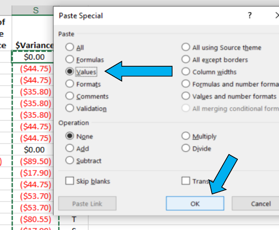
i. Highlight all line in the $variance column (Column S) beginning with Cell S2
ii. With all lines in Column S highlighted, right click and select “Copy”
iii. Right Click on Cell S2 and select “Paste Special”
iv. In the pop-up window that appears, select the button for “Values” in the ‘paste’ section, then
click “OK”. (No other selections in the pop-up window are needed)
v. Delete all columns except for Unique ID and $Variance
vi. Unique ID should remain in Column A with $Variance now occupying Column B.
vii. In the $Variance column, there should either be a $0.00 or a take-back amount
viii. Save As with the new title being the “Provider Name / Audit / Ingest”

2. RAT-STATS – Determine Extrapolation Amount:
a. Under the heading “Estimation” select the “Unrestricted Variable” option
b. A pop-up window will appear
i. Enter the Name of the Audit/Review.
ii. Enter the Frame Size = Total Number of Claim Lines in Scope
iii. Make sure the “Include All Rows” has been checked
iv. Under Data File Format - Select “Difference Values”
v. Next to “Data File” click the “Select” button
vi. Choose the Excel file “Provider Name / Audit / Ingest”
vii. Difference Cell = B2
viii. Check the box next to “Text File” under File Output Options
1. Save the file as “Provider Name / Audit / Case # / Extrapolation Results” in the audit
folder
ix. Click “Process”

x. A final window will appear that gives the details of the audit and extrapolation amount -----
CBH will utilize the amounts displayed in the 90% confidence level column to determine the
total financial impact of the audit.

Appendix A
Name of Audit
Total Number of
Claim Lines in Scope (Universe Size)
Mean
Standard Deviation
Seed Number
Sample Size
(Confidence Level 90%/Sample Precision 5%)
Total $ Amount of Claims in Sample
***For Use in Extrapolation Only***
Total $ Variance Amount
Error Rate (%)
Extrapolation Amount
(Confidence Level 90%)
Lower Limit
Upper Limit
Point Estimate
