Excel magic

By: Mary Jo Webster

@MARYJOWEBSTER, MJWEBSTER71@GMAIL.COM

UPDATED: JANUARY 2019

EXCEL MAGIC

Table of contents:

Date functions

Dealing with time

String functions

Other text functions

IF statements

SUMIF, COUNTIF

Lookups

Miscellaneous

Tableau Reshaper

Hyperlink to documents

Download matching practice data here:

https://mjwebster.github.io/DataJ

- -

Excel Magic

This handout contains a variety of functions and tricks that can be used for cleaning

and/or analyzing data in Excel. This handout refers to data in an Excel file called

“ExcelMagic.xlsx"

Date Functions:

Month-Day-Year (use worksheet called “Dates”):

This is one of my all-time favorite tricks. It works in both Excel and Access. It allows you to grab

just one piece of a date. So if you have a series of dates and you want a new field that just gives

the year. Or if you want a new field to just list the month.

=Year(Datefield)

=Month(Datefield)

=Day(Datefield)

So if you have 4/3/04, here’s what you’ll get with each formula:

Year: 2004

Month: 4

Day: 3 (it gives the date, as in the 3rd day of the month)

Weekday:

This works much the same way as the above formula, but instead it returns the actual day of the

week (Monday, Tuesday, etc). However the results come out as 1 (for Sunday), 2 (for Monday).

=Weekday(Datefield)

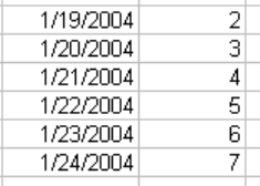
Here’s what the answers look like for one week in January:

Note: If you want the 1 value to represent Monday (then 2 for Tuesday, 3 for Wednesday, et),

add a 2 on to the formula like this:

=weekday(datefield,2)

Displaying words instead of numbers:

Go to Format > Cells and choose Custom and type “ddd” in the Type box provided. It will display

1 as “Sun”, 2 as “Mon”, etc. However, the underlying information will remain the numbers. So if

you want to base an IF..THEN statement on this field or something like that, your formula would

need to refer to the numbers.

- -

DateValue:

If you imported some data and your Date field stayed as text and is not being recognized as a

true date (which is necessary for proper sorting), here’s how you can fix it. The date has to

appear like a real date --- in other words, either 3/4/04 or March 4, 2004 or 4-March-2004 or

one of the other recognized date formats. You can tell that Excel is not recognizing it as a date if

the text is pushed all the way to the left of the cell. See picture:

=DATEVALUE(String)

The String that goes inside the parentheses is the cell where your data starts.

Example: =DATEVALUE(b2)

Datedif

Useful for calculating ages from birthdates. It gives you the difference between two dates in

whatever unit of measure you specify.

=Datedif(Date 1, Date 2, Unit of Measure)

Units of Measure:

“y” --- years

“m” ---months

“ym” ---number of months since the last year

You can use the TODAY() function to refer to today’s date. Or you could put a specific date in

there (with quotes around it)

Examples:

=Datedif(b2,today(), “y”)

=Datedif(b2, “1/1/2004”, “y”)

Weeknum:

This one requires that you have the Analysis ToolPak installed. It is an add-in for Excel. If the

install of Excel was done properly, you should be able to go to the Tools Menu and choose “Add-

ins” and then click the check box next to Analysis ToolPak. If that option is grayed out that

means you need to re-install Excel.

Weeknum returns the number that corresponds to where the week falls numerically during the

year. The formula looks like this:

=Weeknum(celladddress)

- -

Displaying data as a calendar: (use worksheet called “Calendar”)

You can use Weeknum and Weekday (listed above) in conjunction with Pivot Tables to display

data in a sort of calendar form. This would be useful if you’re looking for patterns in your data

based on the calendar.

To do that, you need to add fields to your data with WeekNum and WeekDay corresponding to

the date in that field. Then create a Pivot Table, with WeekNum in the Row, WeekDay in the

Column and whatever field you want to count or sum in the Data box. (I found that you need to

leave the WeekDay output as 1, 2, 3, etc., so that it will display in the proper order. I tried to

have them display as “Mon”, “Tues”, etc and it wouldn’t put them in order)

Response Times (use worksheet called “time”):

One of the most common things journalists want to do with a date/time field is to calculate

response times of local public safety units. To do this, you need to make sure to have full

date/time fields for all the key time points you want to compare (i.e. time of 911 call, dispatch

time, arrival time, cleared time). Be sure that these have dates for each time, as well, because

calls that occur just before midnight might result in an arrival or cleared time occurring on a

different date.

Even if you’re not doing response times, a useful formula you might need would be this one to

strip the time portion off of a date/time field:

=TIME(HOUR(h4),MINUTE(h4),SECOND(h4))

The best approach for calculating a response time is to convert your time into seconds. Here are

the steps you’ll need to do that. (use the worksheet called “TIME” to follow along):

This assumes that you have a date/time field (i.e. “3/31/2013 12:00 PM” or “3/31/2013 14:00”):

=TIME(HOUR(h4),MINUTE(h4),SECOND(h4))*86400

Note: 86400 is the number of seconds in a 24-hour period. So this answer is really representing

the time as the number of seconds that have elapsed since midnight.

If you have response times with just a time—no date (i.e. “12:00 pm), then you can just multiply

that by 86400.

To deal with calls that run across midnight (call received in p.m. and the arrival time is in a.m.),

we need to be able to handle these differently than the other calls. So we need our formula to

be able to check for that.

The simplest would be to have it look to see if the receive date is different than the arrive date.

However, our fields have both date AND time. So it might help if we add new fields that just

hold the dates.

So we’ll create “RECEIVE DATE” AND “ARRIVE DATE” fields and populate them using these

formulas:

=DATE(YEAR(H4),MONTH(H4),DAY(H4))

- -

=DATE(YEAR(J4),MONTH(J4),DAY(J4))

• Note the “DATE” function used here requires you to put the year first, then month, then day. A

little counterintuitive .

Of course, if you’re feeling confident, you could build that date function into the formula below.

It would just make a really long and complex formula.

Now we can calculate the response time – the difference between the receive time and the

arrive time, and display our answer in minutes.

Here’s the formula, then I’ll explain:

=(IF(N4=O4, M4-K4, (86400-K4)+M4))/60

This criteria portion of this IF statement is “N4=O4” – it’s looking to see if the “receive date” and

“arrive date” are on the same day (if not, that’s an indicator that this runs across midnight).

If that’s true, it subtracts M4-K4 (arrive time seconds minus receive time seconds)

If the criteria is false, it subtracts 86400 (number of seconds in a day) from K4 (the receive time)

and then adds the arrive time.

This strange formula puts the receive time and the arrive time into the same time frame to

make it possible to subtract without getting a negative number.

Finally, we have this whole formula surrounded by parentheses and then divide by 60 off the

end. This converts the answer from seconds to minutes.

- -

Text or String Functions:

(use worksheets called “BasicStrings”, “split names” or “split address”)

These are extremely handy tools that you can use for data cleanup (particularly splitting names)

or during analysis. They allow you to grab only a piece of the information in a field based on

certain criteria. These functions are also available in other software, including most SQL

database programs, and coding languages like R and Python. They often work in a similar

fashion but have slight variations in syntax.

LEFT: This tells the computer to start at the first byte on the left side of the field. Then we have

to tell it how many bytes (or characters) to take.

Syntax: LEFT(celladdress, number of bytes to take)

Example: LEFT(B5, 5) --- this will extract the first 5 characters of the contents of cell B5

MID: To use this function, you have to tell the computer which cell to work on, where to start

and where to stop. If you want to take everything that remains in the field, just put a really big

number in that will likely encompass all possibilities.

Syntax: MID(celladdress, byte number to start at, number of bytes to take)

Example: MID(B5,10,4) --- this will start at the 10

byte and take 4 bytes.

SEARCH: This works as a sort of search tool to tell the computer to either start or stop taking a

“string” at a certain character (or space). This is how we can tell the program to split a name

field at the comma, for example. For this type of work, it is used in conjunction with the MID

function. The character you what to find should be enclosed in quotes.

Syntax: SEARCH(“character we want to find”, celladdress)

Example: SEARCH(“,”,B5)

You can combine this with Mid to explain that you either want to start or stop at a

certain character (even if the character isn’t located at the same byte in every record).

EXAMPLE: MID(b5, search(“,”, b5), 100)

**the above example uses the search function to find the “start” position, then tells the

computer to take 100 bytes from there.

EXAMPLE: MID(b5, 10, search(“,”, b5))

**the above example uses search to find the “end” position.

**Note: If you don’t want to include the character that you searched for in your result, use a –1

or +1 just after the search phrase to either go back a space (-1) or move forward and start a

space farther (+1). Here’s an example that will start at the comma, then move one space

forward and take 100 bytes from there:

=mid(b5, search(“,”,b5)+1, 100)

There is also a RIGHT function, which starts at the first byte on the right side of the field and

then you can tell it how many bytes to take. (it isn’t as useful as the others, however)

- -

Basic Strings:

(use the worksheet called “BasicStrings”)

When I teach people how to use string functions, usually the first response I get is: “Why can’t

you just use Text-to-Columns?” This great feature (found under the Data menu) is very handy if

the column you are trying to split is delimited by something. For example, names such as:

“Smith, John”

But sometimes it won’t work and sometimes your data won’t be that neat and tidy. And when

you hit that day, you’ll thank me for teaching you string functions.

The data in this worksheet is an example of that very

situation. This is school district expenditure data that

had been reported to the state through their financial

accounting database called UFARS. Each row is a

“bucket” of expenditures, coded by the revenue source

used (“finance”), by the “program” it was spent on and

by the “object” for the expenditure (i.e. “food”,

“postage”, “salaries”, “health insurance”)

In the first column you can see those codes are all

strung together, separated neatly by dashes. (Yes, the

first two rows only have one of the three types of codes)

I wanted to separate these out into their own columns – finance, program and object.

I tried to do text-to-columns, first by making a copy of that column and dropping it in a blank

column. Then highlighting that column and selecting “Text-to-Columns” from the data menu. I

told Excel, it was delimited by a dash (“other”) and to treat consecutive delimiters as one. It

looked like everything would work perfectly. But then the new columns no longer had the

leading zeros (which are necessary)!

That’s when I realized string functions would save the day.

To get the finance code (the first three digits), I used the LEFT() function.

=LEFT(a6, 3)

To get the program code (the middle code), I used the MID() function. You tell it which cell to

work on, which byte to start on, and then how many bytes to take. (Note: you have to look

carefully to see how many dashes are in there. The second code starts at byte 9)

=MID(a6, 9, 3)

And to get the last code, you can either use MID in the same fashion….

=MID(a6, 16,3)

OR….

You can use the RIGHT function

=RIGHT(a6, 3)

- -

Splitting names:

Dealing with middle initials:

You can make string functions even more versatile by combining in some other Excel functions.

Here we’re going to use the LEN function – which calculates the length of a string – and an IF

function – which allows you to tell Excel to look for certain criteria and to do one thing if the

criteria is met, and something else if it is not.

Previously, we split them into Lastname and Restname – but we have the middle initials lumped

together with the first name. Here we’re going to separate those out.

First we need to assess whether we have a consistent pattern we can rely on. In most of these

records, you’ll see we have either a solo first name or a first name with a middle initial. You’ll

also want to make sure they are consistent in terms of periods – are there either no periods on

all records? Or periods on all records? The formula we’re going to use below assumes there are

no periods. And if you’re at all unsure about whether periods exist in your data, I’d recommend

doing a replace-all to get rid of them before you try to split the names.

We also need to keep an eye out for any other variations, especially around the middle initial.

Here we have one record that breaks the pattern – Alex Baldwin has his suffix in there.

“Alexander R III”

Since we don’t have very many records with a suffix, here we’re going to just edit those by hand.

If you had a very large dataset and you don’t know where they all are, there are various

techniques for finding the suffixes and separating them off into a new field. My quick

recommendation would be to use a VLOOKUP to find all the variations, isolate those records and

then use a string function (much like we’re doing here) to split them out.

So for now, I’m going to create a suffix field and edit the Alex Baldwin record by hand.

The logic we’re going to use here is to first figure out how long – or how many bytes – each

name consists of (including the middle initial). Then we’re going to “test” whether or not the

second to last byte is a space – if so, we’re going to assume that there’s a middle initial on the

end.

The way to measure how many bytes of data are in a cell is a function called “LEN”

Let’s try it out….

=len(d3)

(Note: you would probably want to check for leading or trailing spaces first and get rid of them

by either creating a new column using the TRIM function --- =trim(d3) --- or by cleaning up the

data in a program like OpenRefine)

This function returns the number of bytes. If you look at Tom Hanks, for example, it says the

restname cell is 5 bytes. That’s 3 bytes for “Tom”, 1 byte for the space and 1 byte for his middle

initial.

- -

(If you haven’t yet used IF functions, skip ahead to that section of this tipsheet and learn how to

use those first)

We’re also going to name our columns so that we can

use those names, instead of cell addresses in our

formulas. Highlight the data in the column with the

“restname” (include the column label) and right-mouse

click and choose “Define Name”.

In the dialog box that comes up (see image), you’ll see

that it guesses you want to call this RESTNAME – if you

included the column label in the section you highlighted.

You can choose to name it something else, though, if

you want. Make sure that the “Refers to” section is

covering the full extent of your data. Click OK.

We can now combine the LEN function, with a MID function and an IF function to test whether

or not there’s a space there. This step is just to show you how it works. (Anywhere that it says

“RESTNAME” is referring to the named label we just created)

=IF(MID(RESTNAME, LEN(RESTNAME)-1, 1)=””, “TRUE”, “FALSE”)

Remember IF statements have three parts – the criteria to look for, what to do if it’s true and

what to do if it’s false.

The formula – MID(RESTNAME, len(RESTNAME)-1, 1)=”” --- is our criteria part. The LEN function

minus 1 tells MID where to start and then we say just grab that one byte. And it’s testing

whether or not that one byte equals a space.

If it does equal a space, we’re dropping the word “true” into our column and if it does not, we’re

dropping in the word “false”

If you copy it down, you’ll see that it worked perfectly.

So now let’s adjust it to make it actually split apart data.

We can keep almost all the formula – we’re just going to edit the “true” and “false” parts.

We’ll change the true part to the string function that’s needed to put the middle initial in this

column, by putting in RIGHT(RESTNAME,1)

And then we’ll change the false part to just two double-quote marks. This is how you tell it to

leave the cell blank.

=IF(MID(RESTNAME, LEN(RESTNAME)-1, 1)=" ", RIGHT(RESTNAME,1), "")

- -

One last step…let’s put the firstname out to its own column too. We’ll use a similar formula with

just a couple tweaks

We’ll leave the criteria part of the formula the same

=IF(MID(RESTNAME, LEN(RESTNAME)-1, 1)=" ",

Then this time the true portion needs to be what to do if there is a middle initial – in this case

we want to tell it to start on the left and go until it hits the space. Remember that are LEN

formula -1 gives us the spot! And we’ll Trim it just in case.

LEFT(RESTNAME,TRIM(LEN(RESTNAME)-1)),

Then the false portion of our formula is what to do if there is NOT a middle initial. In that case,

we merely want to copy over the contents of the D column. We’ll trim it, just in case.

TRIM(RESTNAME))

Here’s full formula:

=IF(MID(RESTNAME,LEN(RESTNAME)-1,1)=" ",LEFT(RESTNAME,TRIM(LEN(RESTNAME)-

1)),TRIM(RESTNAME))

Be sure to troll through your data and look for anomalies. Use the Filter feature or run a Pivot

Table to look for problem records.

Trick for splitting apart city and state when it’s not delimited

(use worksheet called “citystate”)

This trick is only going to work in specific circumstances, but it’s one you might encounter with

some frequency. Here’s the deal…you’ve got a spreadsheet that has a column containing both

the city name (or perhaps a county name) and a two-digit state abbreviation but there isn’t a

comma separating the two items, so it’s not easy to parse.

You can use the LEN function to determine how long the full string is and then subtract 2 digits

to find out what byte position that last space is at. (since that’s the byte position you want to

use for splitting the info).

So in column B, put in this formula and copy it down:

=len(a2)-2

A2 is the first cell where our data (city-state column) is located. The first part of the formula –

LEN(A2) – is calculating the number of bytes there are in the cell. And then -2 is just subtracting

two bytes.

Check your numbers on a few examples to make sure it’s hitting the right position. Then you can

use that number you just created (in the B column)

To grab the city name:

=LEFT(a2,b2)

- -

See how I substituted “b2” instead of putting the search(“,”, a2) like we did in the example

above?

Then you can grab the state abbreviation either by using:

=RIGHT(A2,2)

=MID(A2,B2,2)

Other text functions:

SUBSTITUTE(cell, oldtext, newtext): Allows you to mass replace (or elimination) of a specific

word or phrase in a column. For example, I have a list of school districts and the names of the

schools all end with “public school district”. But I want to strip that off.

Here’s the formula I used in the above example:

=SUBSTITUTE(a3, “PUBLIC SCHOOL DISTRICT”, “”)

In the above example I’m leaving the “newtext” part of the formula blank because I don’t want

to replace the phrase with something else. If you wanted to change it — perhaps you want it to

say, “Schools” — then you could put that within that last set of quotes.

The function is very specific. For example it won’t replace the phrase “PUBLIC SCHOOL DIST”

because it’s not an exact match.

EXACT(text1, text2): (use worksheet called “Exact”) Compares two strings to see whether they

are identical. This is great for if you are trying to line up two sets of lists. Let’s say each contains

the 50 states, so you want to align them by the name of the state (which appears in both lists). It

returns FALSE if the two items are not identical.

=EXACT(E1, F1)

- -

REPT(text, number): This one is kind of interesting. It repeats the given text whatever number of

times you tell it. The most interesting use of this I found is to generate a sort of bar chart on the

fly. So for example, let’s say you have a list with totals of something in column B.

You could have it create bar charts using the

pipe “|” character based on the total number,

like this:

=REPT(“|”, b2)

When you copy this down to the remaining

rows you’ll see it create a bar for each line.

LEN(text): Returns the length in number of bytes.

PROPER(text): Converts the data in the cell to proper case. LOWER and UPPER are also

available.

- -

IF Statements:

(use worksheets called “BasicIF”, “More BasicIF”)

These are one of several LOGICAL functions that are available in Excel. It’s an extremely

powerful tool for a variety of tasks, most notably for assigning categories to your data based on

certain criteria and for some data cleanup functions that require looking for patterns. Essentially

they allow you to do one thing if your criteria is true, and another thing if your criteria is false.

Later, we’ll talk about nested IF functions that allow you to use multiple criteria.

A basic IF statement consists of:

1) What we’re going to measure as being either true or false

2) What to do if it’s true

3) What to do if it’s false

=IF(criteria, true, false)

Let’s try this out with the “BasicIF” worksheet. This has salary data from the St. Paul police

department. The chief has just announced that everyone is getting a 1% raise, but all will get a

minimum raise of $350 (if 1% of their salary is less than $350).

So for the story, I want to figure out how much additional money this is going to mean (the total

of the “raise” column) based on the current workforce, and then generate a new salary for each

individual.

So the crux of our formula is this: If 1% of the person’s salary is less than $350, then the amount

of their raise will be $350. If not, then it will be 1% of their salary.

As we did earlier, let’s make this easier on ourselves by assigning “names” to our columns and

also the values we’re going to need in our formula

Start by typing $350 in G1 cell at the top of the page. Click on that cell and name it “minimum”

(you can either right-mouse click and choose “define name” or you can go to upper left of the

page and overwrite where it says G1)

And then type 1% in another blank cell—let’s use G2 – and name that one “RaisePct”

Then highlight the whole Salary column (including the label) and name it Salary

Here’s our criteria part:

=if(Salary*RaisePct<Minimum,

- -

Then the true part will just be 350

=if(Salary * RaisePct < Minimum, Minimum,

And the false part will be the salary times 1%

=if(Salary * RaisePct < Minimum, Minimum, Salary * RaisePct)

Now we can add together the original salary and the raise to get their new salary

---------------------

Basic nested IF statements:

In the MoreBasicIF worksheet, let’s look at this data on scores from football games. The data

shows us the scores for the home team and the visit team, but it doesn’t tell us who won the

game.

Since it’s possible for an NFL game to end in a tie (and several did in 2018), let’s first look at

what we’d need to do to figure out if a game ended in a tie. Then we’ll put that together with

another IF statement to create a new field that tells us which team won the game, or if it ended

in a tie.

Let’s just look at the formula we’d need to figure out a tie.

=IF(f2=g2, “tie”, “not tie”)

The criteria portion is simply – “Is the home score equal to the visit score?”

Then the true portion tells it to put the word “tie” in the new field.

And the false portion says to put the words “not tie” in the new field.

- -

But we ultimately want a single field that either says “tie” (for the games that tied), or it has the

name of the winning team.

To get that, we need to “nest” two IF statements together.

First, we need to determine if the game ended in a tie. If that’s true, it will put the word “tie” in

our new field.

If it’s false, Excel will evaluate our second IF statement – if the home score is greater than the

visit score, then grab the name of the home team; if not, then grab the name of the visit team.

In other words, the second IF statement is the “false” portion of our first IF statement.

Here’s what it looks like….

=IF(f2=g2, “tie”, if( f2>g2 , d2, e2) )

Let’s do one more nested IF statement on this worksheet. I want a column indicating whether

the home team won the game, the visit team won the game or that it ended in a tie.

So our new column will have either “home”, “visit” or “tie” as the values.

Using IF to copy down blank columns:

(use worksheet called “Copy down”)

I use this quite frequently when I get data that lists a team name as a title, then all the players or

all the game dates below that. But I want to apply the team name to each record.

The trick is that you need to have a pattern to follow. In the example below, the pattern is that

the B column is always blank on the lines where the team name is listed. And it’s not blank

anywhere else.

- -

So this formula is going to look to see if the B cell is blank:

=IF(b2= “”, a2,c2)

Then it’s going to put the contents of A2 (in this case, “Arizona Cardinals”) in the field if it finds it

to be true. If it’s not true, it looks to the cell directly above (c2) to essentially copy down the

team name.

Combining other functions:

Now that you know the basics of an IF statement, you can jazz it up with all kinds of other

functions. You just place the function as either the criteria, the true part or the false part. Of

course, you can use multiple functions in the same IF statement if necessary.

Examples (I’ve just made these up!):

If a date (located in b2) is for a Monday, then put the word Monday in a new cell, otherwise do

nothing:

=if(weekday(b2)=2, “Monday”, “”)

If a date (located in b2) is equal to another date (located in c2), then put the word “Same” in the

new field, otherwise calculate the difference in months:

=if(b2>c2, “Same”, datedif(b2,c2, “m”))

Using a wildcard search:

You can use the SEARCH function to look for a word or symbol contained within other text,

however it gets a little tricky to make it work properly. You have to add the ISERROR function. If

you want to get in this deep, I recommend checking out the help file on these functions.

Otherwise, here’s a quick hit to get you started:

This example assumes you have a list of cities and states and you

want to flag all of the ones that are in Texas. In this case, the state

name is written out in full.

So if it finds Texas, this formula instructs it to put an X in the C

column, otherwise leave it blank.

=IF(ISERROR(SEARCH("*Texas*",B4,1)>0)=FALSE, "X","")

The criteria part of this stretches from the ISERROR all the way to the FALSE. The ISERROR is

necessary because it will give you an error message if it doesn’t find the word. It’s the only way

you can instruct the computer to do something in the false portion of your answer (even if that

means just leaving it blank).

The following portion:

SEARCH(“*Texas*”, b4, 1)

If used alone, this portion will return a 1 if it finds the search term and an error message if it

doesn’t. So then you need to add the IF portion to give it two options. By adding the ISERROR

and the =FALSE, you can sidestep the error message.

- -

More nested IF statements:

(use worksheet called “NestedIF_2”)

This is data on schools in Minneapolis. It identifies (only by number) the principals at each

school, each year. Some schools have up to 8 years’ worth of data, others have fewer years

because they haven’t been open the whole 8 years. Our goal is to figure out how many different

principals each school has had during this time. We can’t just count the number of records,

cause you’ll just get the number of years’ worth of data we have for each school. There are

quicker ways to do this in SQL, but if you want to stay working in Excel, this is a good solution.

We’ll start by making sure the data is sorted by school number and then by data year,

ascending. The school number is the only consistent identification we have for a school (names

sometimes change from year to year).

Our IF statement is going to first figure out if we’re on the first record for a school or not. If it is

the first record, it will mark that record with a “1” (our first principal). If it’s not, it will do a

second IF statement that looks to see if the person number is the same as the person number in

the row above. If it is the same number, it’ll put a 0 in (since this is not a new principal). If it’s a

different number, it will put in a 1 (a new principal). When we’re finished, we’ll have a column

we can use in a pivot table to SUM the number of principals.

Let’s put our formula in cell F10.

Here’s the first part of our formula (the ellipsis indicates the part we haven’t finished yet)

It’s looking to see if the school number on row 10 is the same as on row 9 and puts in the

number 1 if that’s true. We haven’t gotten to the false portion yet.

=if(d10<>d9), 1, …..)

You’re probably thinking, duh! Row 9 is the header row! Yes, you’re right. But it will make more

sense when you go farther down into your data.

Here’s the full formula:

=if(d10<>d9), 1, if(e10<>e9), 1, 0))

The second IF formula is embedded in the “false” portion of our first IF statement; in other

words, it will only put that formula to use if it’s on a record where the school number matched

the row above.

This second IF formula looks at the person number in column E. It puts the number 1 in if the

person number doesn’t match the row above (a new principal) and puts in 0 if it does match the

row above.

When copy the formula down the page and you look at your results, you should see that there is

always a 1 in the first row for each school (probably the 09-10 school year). And then there

should only be another 1 for that same school if there’s a new principal in a subsequent year.

Now that you have this filled in (make sure there’s a header on that column!) and then you can

build a Pivot Table that has the school number in the rows and SUM of the column F. That will

- -

give you an answer of how many principals each school had. (Some of you may have realized

that you might also want to count up how many years for each school so you can say something

like…. Bryn Mawr had 3 principals in 8 years, while Ramsey Middle had 1 in 3 years.)

Even more complicated nested IF statements:

(use worksheet called “Nested IF”)

The sheet in ExcelMagic called “Nested IF” has data from Minnesota’s gay marriage battle. It has

one record for each state house district. Then in columns B through G we have results from a

2012 statewide ballot measure calling for a ban on gay marriage. The last three columns indicate

the legislator in that district in 2013, their party affiliation (DFL=Democrat) and how they voted

on a bill in 2013 that allowed gay marriage. (Ultimately the bill was signed into law).

The goal here was to find legislators who were not in sync with their district on this issue.

Political analysts were saying these would be the legislators who would be targeted by the

opposing party in the next round of elections.

So there are two things we can do here:

1) First, let’s identify which districts approved the ballot measure (PctYes>.5) or not.

2) Second, let’s identify which legislators voted the opposite of their constituents.

3) Then, of the ones who were opposite of their constituents, which districts either passed

or opposed the 2012 ballot measure by a large margin (60% or more)

Step 1 – In the “Ballot Result” column, let’s identify whether ballot measure passed (Y) or not (Y)

or if there was a tie (TIE)

We’ll need a nested IF statement to do that. Remember that an IF statement is made up of 3

parts – the criteria (Excel calls it the “logical test”), what to do if it’s true, and what to do if it’s

false. When you “nest” an IF statement you just drop it into either the true spot or the false spot

of the first IF statement.

So in this example, I want to see if the PctYes was greater than 50%, and put “Y” in our column if

that’s true. If that’s false, then I want to check for a tie and put “tie” in if it’s true, and put “N” in

if that’s false.

=IF(CRITERIA1, TRUE, IF(CRITERIA2, TRUE, FALSE))

**So let’s name some columns to make this easier.

Highlight the E column (PctYes) and right-mouse click and choose “Define Names”. Call this

“PctYes”

Repeat the process for columns I (“LegisVote”) and J (“BallotResult”)—we’ll need those later.

Exact formula for this one:

=IF(PctYes>0.5, “Y”, if(PctYes=0.5, “tie”, “N”))

- -

Step 2 – let’s now identify which district have “opposites” – the legislator voted one way on the

gay marriage bill in 2013 and his/her constituents went the other way on the 2012 amendment.

We’ll use the field we just created (ballot result) and “LegisVote,” which shows how the

legislator voted in 2013 as a yes or no.

The tricky thing about this one is that “Y” on the amendment and “No” on the Legislator’s vote

actually mean the same thing – both are opposed to gay marriage.

I want a new field that says either “opposite”, “both opposed” or “both in favor”

We’re going to use 3 IF statements for this one. There are different ways to set this up, but it

works generally the same way.

=if(LegisVote= “no”, if(BallotResult=”Y”, “both opposed”, “opposite”), if(BallotResult=”N”, “both

in favor”, “opposite”))

Here’s how to interpret this. First it looks to see if there’s a “No” in the LegisVote column (I). If

true, then it looks to see if there’s a “Y” in the Ballot Result column (J). If that’s true that means

both are opposed. (In other words, we had true on first IF and true on second IF). If the Ballot

result column is NOT “Y”, then it’s going to insert “opposite.” (in other words, true on first IF,

but false on second IF).

The third IF statement is actually the FALSE portion of the first IF statement. So that one won’t

even kick in unless I7=”NO” (our first criteria) is false – in other words, the legislator voted “yes”

So in that scenario, the legislator voted “yes” (it failed the first IF statement), so it skips past the

second IF statement and goes to the 3

IF statement to see if the ballot result (J) is “N”. If that’s

true, then it says “both in favor”. If it’s false, then it says “opposite”(legislator voted “yes” and

constituents approved the ban).

- -

An alternative way of doing this would be to use the AND() function. This allows you to have 2

criteria in the same IF statement. In this, we’re going to nest 2 IF statements, both using the

AND function.

Here’s how the AND fits into an IF statement:

=IF(AND(criteria1, criteria2), true, false)

Here’s the formula we’ll use for this one:

=if(AND(LegisVote=”yes”, BallotResult=”N”), “both in favor”, if(AND(LegisVote=”no”,

BallotResult=”Y”), “both opposed”, “opposite”))

This first looks to see if the legislators and constituents are both in favor, if that’s false then it

looks to see if they are both opposed. And then if that’s ALSO false (now we’ve got 2 false Ifs),

then it says there’s an “opposite” going on.

Using IF functions to re-arrange data

(Use worksheet called “crime”)

One of the most common situations where I use IF statements is to rearrange data that comes

to me in a “report” fashion or has some other problem that makes it difficult or impossible to do

even simple things like sort or PivotTables.

The “crime” worksheet is Uniform Crime Report data that I got from the Minnesota Bureau of

Criminal Apprehension. This is exactly how it came to me.

You can see that there are 5 rows for each jurisdiction, each separated by a blank row. The 5

rows include one that shows total offenses (marked “O”), one that shows total cleared offenses

(marked “C”), one that has the percentage cleared (marked “%”) , one that shows the crimes per

100,000 (crime rate, marked “R”) and then there’s another line that simply has the population

that was used to calculate the crime rate.

The biggest problem with this data, though, is that the identifying information about the

jurisdiction is NOT attached to each row. Each piece of identifying information – name of city or

county, whether it’s sheriff, PD or county total, the ID number for the jurisdiction and the

population – are listed separately on each of the five rows.

- -

So that’s the first problem that needs to be solved before you can rip apart this sheet and re-

arrange to your liking. And IF statements are a great way to fix it.

Step 1:

Create 4 new fields (I put mine on the left side of the data) to hold our identifying information –

city/county, type of jurisdiction, ID number, and population.

Step 2:

IF functions need a pattern in order to work. The pattern we have is that the row marked as “O”

is always the first record for each jurisdiction. So we can essentially use this to tell Excel that it’s

time to switch to a new jurisdiction.

And if the IF statement is on a row that doesn’t have an “O” that means it’s still on the same

jurisdiction it was on in the previous row (with exception of those blank rows, but we don’t care

about those anyway)

Here’s how we’ll set up the first IF statement to populate the new County/City column:

=IF(f9= “O”, E9, A8)

This is saying, if the F column=”O”, then grab the contents of E9 (the name of the county/city), if

it’s not then grab whatever the formula dropped into our new column in the row directly above.

The first line doesn’t make sense – if you look at A8, that’s the header row.

But copy the formula down and then look at the formula in line 10.

- -

Excel automatically adjusted the formula so that it’s now looking at F10 (not F9) and it doesn’t

find an “O”, so instead of grabbing E10 (which is what the formula says would happen if the

criteria is true) it has grabbed A9 – the value that the formula just dropped in the first row.

Go ahead and copy down the whole sheet and you’ll see that it should appropriately switch to a

new jurisdiction each time it encounters an “O” row. But you should check it periodically

throughout the sheet to make sure nothing went wrong somewhere down the line (the only

reason a problem would occur is if the 5 rows per jurisdiction pattern suddenly changes…i.e.

that there are only 4 rows or there are 6 rows per jurisdiction)

Now we can use very similar formulas for the three other columns. The only change is what

piece of info we grab if it’s true or false.

Once you have all four columns populated and checked your work, you can Copy-PasteSpecial-

Values to get rid of the formulas.

Then if you fix the header row (so that it’s all on one row and that all columns have headers),

you can turn on Filter and isolate the records you want to move. For example, you could select

all the “O” records (offenses) and put those in a separate worksheet.

- -

Using IF statements to deal with election data:

(use worksheet “IF_election”)

Election data often comes to us with just raw vote totals for each candidate and no indication of

who won that precinct or county or whatever geography we’re looking at. This solution uses a

combination of various Excel functions – IF, LARGE, MAX, INDEX, MATCH – to give you an

answer.

However, this solution only works if your data is structured so that there is one row for each

geography and the candidate vote totals are in separate columns. (If your data comes with one

row for each candidate – meaning multiple rows for each geography – you can use a Pivot Table

to get it into this structure).

Here’s the big bad formula that we’re going to end up with….

=IF(LARGE(D3:i3,1)>LARGE(d3:i3,2), INDEX($D$2:$i$2,1, MATCH(MAX(D3:i3),D3:i3,0)),"Tie")

But to help you understand how this works, I’m going to break it down into pieces and then put

it together at the end.

First let’s look at this function called LARGE. This allows you to look at an array of data (in this

case, the vote totals for each candidate in a given county) and determine which is the largest, or

second largest, etc.

In a new column on row 3 (where our data starts), type:

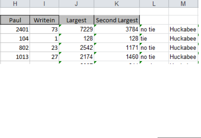
=LARGE(D3:I3, 1)

This will give us the vote total that is the largest out of all the votes. In our example, it is

returning 7,229 for Hennepin County.

In another new column on row 3, type:

=LARGE(D3:I3,2)

This will give us the vote together that is the second largest. It’s giving us 3,784 for Hennepin

County.

If there were a tie -- if two candidates both got 7,229 votes, then the second largest formula

would return that same number.

So we can use those two pieces to test whether or not we’ve got a tie situation. We’ll embed

those two pieces into an IF statement.

- -

Put this in another new column, just to test it out:

=if(LARGE(d3:i3,1)>LARGE(d3:i3,2), “no tie”, “tie”))

That’s going to end up being the core piece of our formula, but instead of dropping the phrase

“no tie” into our worksheet, we want it to give us the name of a winner. So next we need to

build the portion of the formula that we will drop in that spot (where it now says “no tie”)

The first piece of that uses the INDEX function. This allows you to specify an array of data and

have it return a value from a particular row and particular column.

For example:

=INDEX($d$2:$i$2, 1, 3)

This looks at D2 to i2 (and because of the anchors, it will always look at that row when you copy

the formula down) and it will grab whatever is housed in the first row and the third column. If

you try this out in the worksheet, it will return “Huckabee” cause that’s what’s in the third

column of that array.

We’re going to have it reference the header column – where the names are located – so that we

can use that to drop the name of the winner into our data. (Just make sure the header row has

the names the way you want them! In my example, I’m just using their last names.)

But we don’t want our final formula to be hard-coded like that to just the third column (it always

says “Huckabee”!!). We want that value – referring to the column – to change depending who

has the biggest vote total.

That’s where the MATCH function comes in.

MATCH lets you compare two things and it will return the column number where it finds the

match. So in this case, we want to find the biggest value out of the vote totals (remember, that

we’ve already screened out any possible ties – this formula will only do its work on rows where

there is not a tie).

The MAX function will tell us the biggest between columns d and i.

=MAX(d3:i3)

Let’s add that into a MATCH function—it will become the first argument (i.e. the “Lookup

value”)

- -

=MATCH(MAX(d3:i3), d3:i3, 0)

The second argument in our function --- “d3:i3” – is the “lookup array” – in other words, this is

the range of cells where MATCH is going to look to find the same value that matches the value

returned by Max(d3:i3)

The zero at the end of the MATCH formula is merely telling Excel to only do an EXACT match.

(I.e. the “match type”)

If you try this out in the spreadsheet, it will return the number 4 for Hennepin County. In other

words, the 4

column in our array (the column for Romney) has the biggest value.

Now let’s look back at the INDEX function. Remember that you have to tell Index which column

number to go to. In the example above, we hard-coded it to the 3

column. But instead, we can

drop this MATCH function into that space in our formula and get the correct answer for each

row of our data.

Try this out in a new column:

=INDEX($D$2:$I$2,1, MATCH(MAX(D3:I3),D3:I3,0))

You’ll see that this is working, but if you copy it all the way down, you’ll get wrong answers for

the ones that have ties. So now we can put all our pieces together, to deal with those ties.

=IF(LARGE(D3:i3,1)>LARGE(d3:i3,2), INDEX($D$2:$i$2,1, MATCH(MAX(D3:i3),D3:i3,0)),"Tie")

This formula will work regardless of how many candidates you have. Just adjust the ranges

(d3:i3 or d2:i2) to match the ranges in your worksheet.

Lookup Tables:

(use worksheets called “lookups”, “lookup2”)

The VLOOKUP and HLOOKUP functions allow you to use Excel more like a relational database

program. So if you haven’t made the leap to Access yet, here’s how you can get more

functionality out of Excel.

Both functions are useful for cases where you have data that relates to another chunk of data,

with one field in common. They work best if you have the data in the same workbook, but it can

be on separate worksheets. This might be the list of 50 states with current Census estimate data

in one worksheet and the same list with last year’s data in another worksheet. Or it might be a

one-to-many relationship where you have a list of cell phone calls and another table that groups

the time of day into categories (such as morning, evening and afternoon).

The difference between VLOOKUP and HLOOKUP is that VLOOKUP will troll through your lookup

table vertically (all in one column). HLOOKUP goes through it horizontally, or all in one row.

To demo this, we’ll use a very simple example. One worksheet has data from the Census County

Business Patterns, but each record is only identified by the county FIPS number. I want to add a

field that shows the county name. A second worksheet has the names associated with the FIPS

numbers.

- -

VLOOKUP requires that the field you’re matching on is the

farthest left column of the lookup table, like in my example

pictured here. (Below I’ll show you how to use different

functions if your table is not set up this way).

In this example, my Business Patterns data is in one

worksheet and this lookup table is in a worksheet called

“Lookup2”. Our formula will need to reference that name, so

it’s a good idea to name your worksheets when you do this.

Here’s the structure for VLOOKUP:

VLOOKUP(cell, range of lookup table, column number,

range_lookup)

The cell is the first cell in your data table. In this case it would be the cell containing the first FIPS

number I want to look up.

Range of lookup table is the upper left corner of your lookup table to the lower right corner,

encompassing all fields. In the example pictured above, it would be worded like this:

Lookup2!$A$3:$B$89

“Lookup2!” is how we refer to the other worksheet, then you need to anchor ($) the starting cell

(A3) and ending cell (B89).

The column number refers to the column number of your lookup table that you want to return

in your data. In this case, I want column 2, which contains the name of the county.

For range_lookup you either put TRUE or FALSE. True will first search for an exact match, but

then look for the largest value that is less than your data value. FALSE will only look for an exact

match. In this case we want to use FALSE. You’ll see below when you would want to use True.

So here is our final formula:

=VLOOKUP(B3, Lookup2!$A$3:$B$89,2, FALSE)

Name your lookup: You can simplify this formula by naming your lookup table. Highlight

the cells in your lookup table, in this case A3 to B89. Go to the Insert Menu and choose

Name, then choose Define. Then type in a name (all one word). For this example, let’s

say I called it “FIPSlkup”.

Then you can change your formula to this:

=VLOOKUP(B3, FIPSlkup, 2, FALSE)

- -

VLOOKUP for inexact match:

(use worksheet called “classify”)

This is crime report data that tells me the date and time of the incident, but I want to

add a column that identifies which police shift the call came in on. I’ve heard that some

shifts are particularly bad about ignoring calls that come in just before shift change. So

I’ve created a table indicating the start of each shift.

Note that I have the night shift in there twice. That’s because I need to tell Excel what to

do with the times that occur just after midnight. Without that, Excel doesn’t know what

to do with the calls that occur between midnight and 6 am.

Also note another important point --- the table is in chronological order. This is

important when you’re doing an inexact match.

The reason is that Excel is going to take the time of each call and compare it to this

lookup table, first determining whether it falls at or after 12:00 am, but before 6 a.m. If

not, then it will move down to the next one.

The only thing different in this VLOOKUP formula compared to the first one we did is

that the final argument is TRUE.

- -

MATCH and INDEX:

As I mentioned above, there is another option if your lookup

table is set up differently. Let’s say the FIPS table starts with

the state name and state FIPS in the first two columns, then

has the county FIPS number in the 3rd column. (this is the

worksheet “lookup3”) Obviously VLOOKUP won’t work

because of the placement of that county FIPS column.

Instead you can use a combination of INDEX and MATCH functions. Let’s break it apart first to

see how it works.

Index will go to the data range specified and return the value at the intersection of the row

number and the column number that you provided to it. So, using this alone requires that we

provide specific column and row numbers.

To simplify our formulas, let’s name our lookup table. Highlight the whole table in the

worksheet called “Lookup3” and right-mouse click and choose “define name” – change the

name to “FIPS”

We’ll go back to the worksheet called “Lookup” to do our work.

We could use this formula to get it to return “Anoka”, which is in the 3rd row (the header counts

as a row) of the FIPS lookup table and the fourth column. Just try out this formula on the first

row and see what happens

=INDEX(FIPS, 3,4)

But when trying to match this back to the big data table for all the records, we need more

flexibility. So instead of hard-coding the row number, we’re going to drop the MATCH function

into its place.

We need Match to just look in the C column (where the county FIPS codes are stored), so let’s

name that column. In the lookups3 worksheet, highlight the C column, right-mouse click and

choose “define name.” Let’s call this “FIPScode”

=MATCH(FIPScode, FALSE)

So this is going to the C column (FIPScode) and by setting FALSE, we are saying we want an exact

match.

Here’s the final formula:

=INDEX(FIPS, MATCH(B3, FIPScode, FALSE) ,4)

- -

Remember that the 4 at the end of our formula is referring to the 4

column in our lookup table.

B3 is the column in our big data table – in worksheet “lookups” – that has the FIPS code that we

are matching to the lookup table. (you could name this column and replace the B3 with a name,

if you want)

Misc:

Anchors:

When you need to use an anchor ($) in a formula, here’s a quick way to insert it without a lot of

typing. So here’s an example. Let’s say you need to do a percent of total, like in the example

below. Type the formula without the anchors

=b2/b8

And then push the F4 key. It will insert the $ to lock the B8 cell. This locks it so that it won’t

change if you copy the formula down, or copy across.

A bit more about anchors…..If you want to allow the column to change but not the row, you

would only use the anchor in front of the number. If you want to allow the row to change, but

not the column, then you only use the anchor in front of the column letter.

Rank:

This is a more sophisticated way to rank your records and to account for ties.

=RANK(This Number, $Start Range$:$End Range$, Order)

• This Number should be the cell where your data starts.

• Start Range should be the cell where your data starts. Anchor with dollar signs.

• End Range should be the last cell of your data. Anchor with dollar signs.

- -

• Order is either a 1 (smallest value will get assigned #1) or a 0 (largest value will get

assigned #1).

Example: =RANK(B2,$B$2:$B$100,1)

PercentRank:

Returns the rank — or relative standing - within the dataset as a percentage. So for example, if

you had a list of the payrolls for all of the Major League Baseball Teams, you could do a percent

rank on the payroll to find out which team (the Yankees, of course) have the greatest

percentage of the total.

=PERCENTRANK(array, x, significance)

Array: The range of data that you want to compare each item to

X: the value for which you want to know the percent rank

Significance: an optional value that allows you to set the number of digits

Example:

=PERCENTRANK($a$2:$a$30, a2, 2)

Also check out PERCENTILE and QUARTILE functions in the Help file.

Round:

=ROUND(cell, num_digits): For this one you tell it which cell to do its work on and then the

number decimals you want to round to. For the num_digits you can use something like this.

These examples show how it would round the number 1234.5678

 0 puts it to the nearest integer (1235)

 1 goes to one decimal place (1234.6)

 -1 goes to the nearest tenth (1230)

 -2 to the nearest hundreth (1200)

 -3 to the nearest thousandth. (1000)

Copying down a single date:

Excel’s wonderful feature of copying down (or across) formulas becomes a bit of a nightmare

when you simply want to copy down the same date. Excel will think you want to go on to the

next day, then the next, and the next, etc. Here’s the trick for disabling that:

**Hold down the Control (Ctrl) key while dragging/copying down the first instance of the date.

- -

Using column names instead of cell addresses:

Are you sick of typing cell addresses? You can set up your worksheet so that the headers you’ve

typed for each column can be used as cell addresses in your formulas instead. Here’s how it

works…. First thing to do is make sure your headers are all filled out, that they are single words

(no spaces, no punctuation), and that they are stored on the first line of your worksheet. Next,

highlight all of your data (my favorite way to do this is to put your cursor somewhere in your

dataset and hit Control-Shift-Asterisk).

Go to the Formulas ribbon and look for “Name Manager” and a button that says “Create from

selection.” In the dialog box that comes up make sure that ONLY the “top row” choice is

selected.

Once this is set you can use your field names instead of cell addresses by simply typing the

column name instead of the cell address. So for example, our basic nested IF formula that

looked at NFL game scores, could use cell names instead of the addresses, like this:

You can click on “Name Manager” in the formulas ribbon to see which names you’ve already

defined (and delete any you don’t want)

Understanding Errors:

#DIV/0! : This almost always means the formula is trying to divide by zero or a cell that is blank.

So to fix this, first check to make sure that your underlying data is correct. In many cases, you

will have zeros. For example, the number of minority students in some schools in Minnesota

might be zero, so I have to use an IF statement whenever trying to calculate the percentage of

minority students. Here’s how I get around the error, assuming the number of minority students

is in cell B2 and the total enrollment is in C2. If the number of minority students is greater than

zero, it does the math. Otherwise it puts zero in my field.

=if(b2>0, b2/c2, 0)

#N/A: This is short for “not available” and it usually means the formula couldn’t return a

legitimate result. Usually see this when you use an inappropriate argument or omit a required

argument. Hlookup and Vlookup return this if the lookup value is smaller than the first value in

the lookup range.

#NAME?: You see this when Excel doesn’t recognize a name you used in a formula or when it

interprets text within the formula as an undefined name. In other words, you’ve probably got a

typo in your formula.

- -

#NUM!: This means there’s a problem with a number in your formula (usually when you’re using

a math formula).

#REF!: Your formula contains an invalid cell reference. For example, it might be referring to a

blank cell or to a cell that has since been deleted.

#VALUE!: Means you’ve used an inappropriate argument in a function. This is most often caused

by using the wrong data type.

Tableau Reshaper Tool (only works in Windows Excel 2007 and newer):

Download here and follow the directions to install in Excel :

http://kb.tableausoftware.com/articles/knowledgebase/addin-reshaping-data-excel

This is a great tool for “normalizing” data, whether you plan to put it into Tableau Public

(visualization software) or not.

Let’s start with the worksheet called “Reshaper1.” This has enrollment data from the University

of Minnesota, broken down by race, gender, ethnicity and residency status. For a visualization,

like Tableau, or even some analysis purposes, it would be better to have the data lined up with

one item (or group total) per line – and keep the grand total attached to each group. Like this:

Year GrandTotal Group Value

1997 32342 Men 15470

1997 32342 Women 15872

Etc.

Tableau Reshaper is perfect for this.

First, a little prep work to make this work the best.

• Make sure the headers that are on your columns (in this case, the group names) are

presented EXACTLY as you want them to appear in the final data.

• Make sure that the columns you want to convert are all on the right side of your

spreadsheet and the columns that you want attached to each row are all on the left

side.

Then to make the reshaper tool work, you

put your cursor on the first cell that you want

converted (notice on the screen capture

above, my cursor is on C10 – the first piece of

data I want to put in rows).

Finally, go to the Tableau menu (which was

added to your menu options when you

installed it) and choose “Reshape Data”. It

will ask what cell you want to start with – and

since you put your cursor there previously, it

should guess correctly.

- -

EXAMPLE 2:

For this next one, use the “Reshaper2” worksheet:

Below is an image of data from one of the health insurance exchanges set up under the

Affordable Care Act. Each row is an insurance product offered in a particular rating area

(geographic area). The premium costs are listed by age, going across the columns (age 0-20, 21,

22, 23, etc)

To analyze this data – and present it in a visualization – I want each age to have its own row. So

instead of one row for each insurance product in a rating area, we’ll end up with 45 (there are

45 age groups in this data)

To reshape, put your cursor on the first data point – in this case F2 – and push the “Reshape

Data” button under the Tableau ribbon.

It will push the data out to a new worksheet.

Note: If the new data file exceeds 1 million rows, this will automatically export your results as a

.CSV file

- -

Build hyperlinks with a formula

(use worksheet called “hyperlinks”

These directions are geared for a Windows machine. But it’s likely that with a tweak or two, it

will work for Mac as well. More details:

https://www.contextures.com/excelhyperlinkfunction.html#formulawritten

A colleague of mine got data on condemnations in the city. Each record in the spreadsheet had

basic information about the house that got condemned, but then there was also a Word

document for each one containing a copy of the letter the city sent to the occupants.

The spreadsheet included a column with the name of the Word document that matched each

record. All the names were something like this: 4317705_3396272_14084914.doc

She asked me if there was a way to hyperlink to each of those documents, so she could launch

open the Word document right from Excel. Yes, there is! And this will work whether you are

linking to Word documents, other Excel files or PDFs. The key is that the name and the file

extension (.doc, .docx, .xlsx, .pdf, etc) be listed with the name of the file. (If it’s not, you can you

concatenate to tack it on in a new column of your spreadsheet)

Another helpful thing is that you should have your spreadsheet and the documents stored near

each other. These directions will show you what I’d recommend as best practice – that the

documents be stored in a sub-directory of the folder where you have the spreadsheet.

So, for this example, let’s say our main folder is called “condemn”. And our spreadsheet is in

that folder.

Make a sub-folder inside “condemn” and call it “documents” and put all those Word documents

in that directory.

/condemn/documents

Then go into your spreadsheet and create a new column where you will put the hyperlink.

We’ll use an Excel function called HYPERLINK(), which has 2 arguments. The first is the path to

the document. The second is the name you want to appear on the URL you are creating.

Notice below, I’ve highlighted in yellow the first argument – the file path. You can see that we

are hard-coding the path, then concatenating (&) that with the contents of E2, which contains

the file name. We want that to change as we copy the formula down the data.

Also note that the path has a period at the front of it to tell Windows to go into a sub-directory.

=HYPERLINK(“.\documents\” & E2, E2)

The second argument – in this case, the second instance of E2, is simply telling it what to display

when the URL appears on the worksheet. I’m just telling it to display the file name. You could do

something like this and it would say “open document” for every row:

=HYPERLINK(“.\documents\” & E2, “open document”)