
Suitable for both beginners and advanced users, Dynamic Documents
with R and knitr, Second Edition makes writing statistical reports eas-
ier by integrating computing directly with reporting. Reports range from
homework, projects, exams, books, blogs, and Web pages to virtually any
documents related to statistical graphics, computing, and data analysis.
The book covers basic applications for beginners while guiding power us-
ers in understanding the extensibility of the knitr package.
New to the Second Edition
• A new chapter that introduces R Markdown v2
• Changes that reect improvements in the knitr package
• New sections on generating tables, dening custom printing methods
for objects in code chunks, the C/Fortran engines, the Stan engine,
running engines in a persistent session, and starting a local server to
serve dynamic documents
Like its highly praised predecessor, this edition shows you how to improve
your efciency in writing reports. The book takes you from program output
to publication-quality reports, helping you ne-tune every aspect of your
report. Demos and other information about the package are available on
the author’s website.
Yihui Xie is a software engineer at RStudio. He earned a PhD from the
Department of Statistics at Iowa State University. His research focuses on
interactive statistical graphics and statistical computing. He is an active
R user and the author of several award-winning R packages. He is also
the founder of “Capital of Statistics,” a large online statistics community
in China.
K25425
w w w
.
c r c p r e s s
.
c o m
The R Series
Dynamic Documents
with R and knitr
Second Edition
Dynamic Documents with R and knitr
Yihui Xie
Xie
Second
Edition
Statistics
K25425_cover.indd 1 4/17/15 11:01 AM

Yihui Xie
RStudio, Inc.
Dynamic Documents
with R and knitr
Second Edition
Chapman & Hall/CRC
The R Series
John M. Chambers
Department of Statistics
Stanford University
Stanford, California, USA
Duncan Temple Lang
Department of Statistics
University of California, Davis
Davis, California, USA
Torsten Hothorn
Division of Biostatistics
University of Zurich
Switzerland
Hadley Wickham
RStudio
Boston, Massachusetts, USA
Aims and Scope
This book series reects the recent rapid growth in the development and application
of R, the programming language and software environment for statistical computing
and graphics. R is now widely used in academic research, education, and industry.
It is constantly growing, with new versions of the core software released regularly
and more than 6,000 packages available. It is difcult for the documentation to
keep pace with the expansion of the software, and this vital book series provides a
forum for the publication of books covering many aspects of the development and
application of R.
The scope of the series is wide, covering three main threads:
• Applications of R to specic disciplines such as biology, epidemiology,
genetics, engineering, nance, and the social sciences.
• Using R for the study of topics of statistical methodology, such as linear and
mixed modeling, time series, Bayesian methods, and missing data.
• The development of R, including programming, building packages, and
graphics.
The books will appeal to programmers and developers of R software, as well as
applied statisticians and data analysts in many elds. The books will feature
detailed worked examples and R code fully integrated into the text, ensuring their
usefulness to researchers, practitioners and students.
Series Editors
Published Titles
Stated Preference Methods Using R, Hideo Aizaki, Tomoaki Nakatani,
and Kazuo Sato
Using R for Numerical Analysis in Science and Engineering, Victor A. Bloomfield
Event History Analysis with R, Göran Broström
Computational Actuarial Science with R, Arthur Charpentier
Statistical Computing in C++ and R, Randall L. Eubank and Ana Kupresanin
Reproducible Research with R and RStudio, Second Edition, Christopher Gandrud
Introduction to Scientific Programming and Simulation Using R, Second Edition,
Owen Jones, Robert Maillardet, and Andrew Robinson
Nonparametric Statistical Methods Using R, John Kloke and Joseph McKean
Displaying Time Series, Spatial, and Space-Time Data with R,
Oscar Perpiñán Lamigueiro
Programming Graphical User Interfaces with R, Michael F. Lawrence
and John Verzani
Analyzing Sensory Data with R, Sébastien Lê and Theirry Worch
Parallel Computing for Data Science: With Examples in R, C++ and CUDA,
Norman Matloff
Analyzing Baseball Data with R, Max Marchi and Jim Albert
Growth Curve Analysis and Visualization Using R, Daniel Mirman
R Graphics, Second Edition, Paul Murrell
Data Science in R: A Case Studies Approach to Computational Reasoning and
Problem Solving, Deborah Nolan and Duncan Temple Lang
Multiple Factor Analysis by Example Using R, Jérôme Pagès
Customer and Business Analytics: Applied Data Mining for Business Decision
Making Using R, Daniel S. Putler and Robert E. Krider
Implementing Reproducible Research, Victoria Stodden, Friedrich Leisch,
and Roger D. Peng
Graphical Data Analysis with R, Antony Unwin
Using R for Introductory Statistics, Second Edition, John Verzani
Advanced R, Hadley Wickham
Dynamic Documents with R and knitr, Second Edition, Yihui Xie
CRC Press
Taylor & Francis Group
6000 Broken Sound Parkway NW, Suite 300
Boca Raton, FL 33487-2742
© 2015 by Taylor & Francis Group, LLC
CRC Press is an imprint of Taylor & Francis Group, an Informa business
No claim to original U.S. Government works
Version Date: 20150519
International Standard Book Number-13: 978-1-4987-1697-0 (eBook - PDF)
This book contains information obtained from authentic and highly regarded sources. Reasonable
efforts have been made to publish reliable data and information, but the author and publisher cannot
assume responsibility for the validity of all materials or the consequences of their use. The authors and
publishers have attempted to trace the copyright holders of all material reproduced in this publication
and apologize to copyright holders if permission to publish in this form has not been obtained. If any
copyright material has not been acknowledged please write and let us know so we may rectify in any
future reprint.
Except as permitted under U.S. Copyright Law, no part of this book may be reprinted, reproduced,
transmitted, or utilized in any form by any electronic, mechanical, or other means, now known or
hereafter invented, including photocopying, microfilming, and recording, or in any information stor-
age or retrieval system, without written permission from the publishers.
For permission to photocopy or use material electronically from this work, please access www.copy-
right.com (http://www.copyright.com/) or contact the Copyright Clearance Center, Inc. (CCC), 222
Rosewood Drive, Danvers, MA 01923, 978-750-8400. CCC is a not-for-profit organization that pro-
vides licenses and registration for a variety of users. For organizations that have been granted a photo-
copy license by the CCC, a separate system of payment has been arranged.
Trademark Notice: Product or corporate names may be trademarks or registered trademarks, and are
used only for identification and explanation without intent to infringe.
Visit the Taylor & Francis Web site at
http://www.taylorandfrancis.com
and the CRC Press Web site at
http://www.crcpress.com

To my parents
Shaobai Xie and Guolan Xie


Contents
Preface xiii
Author xxi
List of Figures xxiii
List of Tables xxvii
1 Introduction 1
2 Reproducible Research 5
2.1 Literature . . . . . . . . . . . . . . . . . . . . . . . . . . . 5
2.2 Good and Bad Practices . . . . . . . . . . . . . . . . . . . 7
2.3 Barriers . . . . . . . . . . . . . . . . . . . . . . . . . . . . 9
3 A First Look 11
3.1 Setup . . . . . . . . . . . . . . . . . . . . . . . . . . . . . . 11
3.2 Minimal Examples . . . . . . . . . . . . . . . . . . . . . . 12
3.2.1 An Example in L
A
T
E
X . . . . . . . . . . . . . . . . . 12
3.2.2 An Example in Markdown . . . . . . . . . . . . . 15
3.3 Quick Reporting . . . . . . . . . . . . . . . . . . . . . . . 17
3.4 Extracting R Code . . . . . . . . . . . . . . . . . . . . . . 17
4 Editors 19
4.1 RStudio . . . . . . . . . . . . . . . . . . . . . . . . . . . . 19
4.2 L
Y
X . . . . . . . . . . . . . . . . . . . . . . . . . . . . . . . 23
4.3 Emacs/ESS . . . . . . . . . . . . . . . . . . . . . . . . . . 25
4.4 Other Editors . . . . . . . . . . . . . . . . . . . . . . . . . 26
5 Document Formats 27
5.1 Input Syntax . . . . . . . . . . . . . . . . . . . . . . . . . 27
5.1.1 Chunk Options . . . . . . . . . . . . . . . . . . . . 28
5.1.2 Chunk Label . . . . . . . . . . . . . . . . . . . . . 29
5.1.3 Global Options . . . . . . . . . . . . . . . . . . . . 30
5.1.4 Chunk Syntax . . . . . . . . . . . . . . . . . . . . 30
vii

viii Contents
5.2 Document Formats . . . . . . . . . . . . . . . . . . . . . . 31
5.2.1 Markdown . . . . . . . . . . . . . . . . . . . . . . 31
5.2.2 L
A
T
E
X . . . . . . . . . . . . . . . . . . . . . . . . . . 35
5.2.3 HTML . . . . . . . . . . . . . . . . . . . . . . . . . 35
5.2.4 reStructuredText . . . . . . . . . . . . . . . . . . . 36
5.2.5 AsciiDoc . . . . . . . . . . . . . . . . . . . . . . . 36
5.2.6 Textile . . . . . . . . . . . . . . . . . . . . . . . . . 37
5.2.7 Customization . . . . . . . . . . . . . . . . . . . . 37
5.3 Output Renderers . . . . . . . . . . . . . . . . . . . . . . 39
5.4 R Scripts . . . . . . . . . . . . . . . . . . . . . . . . . . . . 43
6 Text Output 45
6.1 Inline Output . . . . . . . . . . . . . . . . . . . . . . . . . 45
6.2 Chunk Output . . . . . . . . . . . . . . . . . . . . . . . . 46
6.2.1 Chunk Evaluation . . . . . . . . . . . . . . . . . . 46
6.2.2 Code Formatting . . . . . . . . . . . . . . . . . . . 47
6.2.3 Code Decoration . . . . . . . . . . . . . . . . . . . 47
6.2.4 Show/Hide Output . . . . . . . . . . . . . . . . . 49
6.2.5 Collapse Output . . . . . . . . . . . . . . . . . . . 51
6.2.6 Trim Blank Lines . . . . . . . . . . . . . . . . . . . 52
6.3 Tables . . . . . . . . . . . . . . . . . . . . . . . . . . . . . 52
6.4 Automatic Printing . . . . . . . . . . . . . . . . . . . . . . 55
6.5 Themes . . . . . . . . . . . . . . . . . . . . . . . . . . . . 56
7 Graphics 59
7.1 Graphical Devices . . . . . . . . . . . . . . . . . . . . . . 60
7.1.1 Custom Device . . . . . . . . . . . . . . . . . . . . 60
7.1.2 Choose a Device . . . . . . . . . . . . . . . . . . . 60
7.1.3 Device Size . . . . . . . . . . . . . . . . . . . . . . 61
7.1.4 More Device Options . . . . . . . . . . . . . . . . 61
7.1.5 Encoding . . . . . . . . . . . . . . . . . . . . . . . 62
7.1.6 The Dingbats Font . . . . . . . . . . . . . . . . . . 64
7.2 Plot Recording . . . . . . . . . . . . . . . . . . . . . . . . 64
7.3 Plot Rearrangement . . . . . . . . . . . . . . . . . . . . . 69
7.3.1 Animation . . . . . . . . . . . . . . . . . . . . . . 70
7.3.2 Alignment . . . . . . . . . . . . . . . . . . . . . . 71
7.4 Plot Size in Output . . . . . . . . . . . . . . . . . . . . . . 72
7.5 Extra Output Options . . . . . . . . . . . . . . . . . . . . 73
7.6 The tikz() Device . . . . . . . . . . . . . . . . . . . . . . . 74
7.7 Figure Environment . . . . . . . . . . . . . . . . . . . . . 76
7.8 Figure Path . . . . . . . . . . . . . . . . . . . . . . . . . . 78

Contents ix
8 Cache 81
8.1 Implementation . . . . . . . . . . . . . . . . . . . . . . . . 81
8.2 Write Cache . . . . . . . . . . . . . . . . . . . . . . . . . . 82
8.3 When to Update Cache . . . . . . . . . . . . . . . . . . . 83
8.4 Side Effects . . . . . . . . . . . . . . . . . . . . . . . . . . 84
8.5 Chunk Dependencies . . . . . . . . . . . . . . . . . . . . 86
8.5.1 Manual Dependency . . . . . . . . . . . . . . . . 86
8.5.2 Automatic Dependency . . . . . . . . . . . . . . . 87
8.6 Load Cache Manually . . . . . . . . . . . . . . . . . . . . 88
8.7 Other Options . . . . . . . . . . . . . . . . . . . . . . . . . 89
9 Cross Reference 91
9.1 Chunk Reference . . . . . . . . . . . . . . . . . . . . . . . 91
9.1.1 Embed Code Chunks . . . . . . . . . . . . . . . . 91
9.1.2 Reuse Whole Chunks . . . . . . . . . . . . . . . . 92
9.2 Code Externalization . . . . . . . . . . . . . . . . . . . . . 93
9.2.1 Labeled Chunks . . . . . . . . . . . . . . . . . . . 93
9.2.2 Line-Based Chunks . . . . . . . . . . . . . . . . . 94
9.3 Child Documents . . . . . . . . . . . . . . . . . . . . . . . 95
9.3.1 Input Child Documents . . . . . . . . . . . . . . . 95
9.3.2 Child Documents as Templates . . . . . . . . . . 96
9.3.3 Standalone Mode . . . . . . . . . . . . . . . . . . 96
10 Hooks 99
10.1 Chunk Hooks . . . . . . . . . . . . . . . . . . . . . . . . . 99
10.1.1 Create Chunk Hooks . . . . . . . . . . . . . . . . 99
10.1.2 Trigger Chunk Hooks . . . . . . . . . . . . . . . . 100
10.1.3 Hook Arguments . . . . . . . . . . . . . . . . . . 101
10.1.4 Hooks and Chunk Options . . . . . . . . . . . . . 101
10.1.5 Write Output . . . . . . . . . . . . . . . . . . . . . 102
10.2 Examples . . . . . . . . . . . . . . . . . . . . . . . . . . . 103
10.2.1 Crop Plots . . . . . . . . . . . . . . . . . . . . . . . 103
10.2.2 rgl Plots . . . . . . . . . . . . . . . . . . . . . . . . 105
10.2.3 Manually Save Plots . . . . . . . . . . . . . . . . . 106
10.2.4 Optimize PNG Plots . . . . . . . . . . . . . . . . . 108
10.2.5 Close an rgl Device . . . . . . . . . . . . . . . . . 109
10.2.6 WebGL . . . . . . . . . . . . . . . . . . . . . . . . 110
11 Language Engines 111
11.1 Design . . . . . . . . . . . . . . . . . . . . . . . . . . . . . 111
11.1.1 The Engine Function . . . . . . . . . . . . . . . . 112
11.1.2 Engine Options . . . . . . . . . . . . . . . . . . . . 113
11.2 Languages and Tools . . . . . . . . . . . . . . . . . . . . . 113

x Contents
11.2.1 C++ . . . . . . . . . . . . . . . . . . . . . . . . . . 113
11.2.2 C/Fortran . . . . . . . . . . . . . . . . . . . . . . . 115
11.2.3 Interpreted Languages . . . . . . . . . . . . . . . 116
11.2.4 Stan . . . . . . . . . . . . . . . . . . . . . . . . . . 118
11.2.5 TikZ . . . . . . . . . . . . . . . . . . . . . . . . . . 120
11.2.6 Graphviz . . . . . . . . . . . . . . . . . . . . . . . 121
11.2.7 Highlight . . . . . . . . . . . . . . . . . . . . . . . 122
11.2.8 Other Engines . . . . . . . . . . . . . . . . . . . . 123
11.3 Persistent Sessions . . . . . . . . . . . . . . . . . . . . . . 124
12 Tricks and Solutions 127
12.1 Chunk Options . . . . . . . . . . . . . . . . . . . . . . . . 127
12.1.1 Option Aliases . . . . . . . . . . . . . . . . . . . . 127
12.1.2 Option Templates . . . . . . . . . . . . . . . . . . 128
12.1.3 Program Chunk Options . . . . . . . . . . . . . . 128
12.1.4 Code in Appendix . . . . . . . . . . . . . . . . . . 130
12.1.5 Local R Options . . . . . . . . . . . . . . . . . . . 131
12.1.6 Dynamic Code . . . . . . . . . . . . . . . . . . . . 131
12.2 Package Options . . . . . . . . . . . . . . . . . . . . . . . 131
12.3 Typesetting . . . . . . . . . . . . . . . . . . . . . . . . . . 132
12.3.1 Output Width . . . . . . . . . . . . . . . . . . . . 132
12.3.2 Message Colors . . . . . . . . . . . . . . . . . . . 133
12.3.3 Box Padding . . . . . . . . . . . . . . . . . . . . . 134
12.3.4 Beamer . . . . . . . . . . . . . . . . . . . . . . . . 135
12.3.5 Suppress Long Output . . . . . . . . . . . . . . . 137
12.3.6 Escape Special Characters . . . . . . . . . . . . . . 138
12.3.7 The Example Environment . . . . . . . . . . . . . 139
12.3.8 The Docco Style . . . . . . . . . . . . . . . . . . . 140
12.4 Utilities . . . . . . . . . . . . . . . . . . . . . . . . . . . . 141
12.4.1 R Package Citation . . . . . . . . . . . . . . . . . . 143
12.4.2 Image URI . . . . . . . . . . . . . . . . . . . . . . 144
12.4.3 Upload Images . . . . . . . . . . . . . . . . . . . . 145
12.4.4 Compile Documents . . . . . . . . . . . . . . . . . 145
12.4.5 Construct Code Chunks . . . . . . . . . . . . . . . 146
12.4.6 Extract Source Code . . . . . . . . . . . . . . . . . 147
12.4.7 Reproducible Simulation . . . . . . . . . . . . . . 150
12.4.8 R Documentation . . . . . . . . . . . . . . . . . . 151
12.4.9 Rst2pdf . . . . . . . . . . . . . . . . . . . . . . . . 151
12.4.10 Package Demos . . . . . . . . . . . . . . . . . . . 152
12.4.11 Pretty Printing . . . . . . . . . . . . . . . . . . . . 152
12.4.12 A Macro Preprocessor . . . . . . . . . . . . . . . . 155
12.4.13 Exit Knitting Early . . . . . . . . . . . . . . . . . . 156
12.4.14 Literal knitr Source Code . . . . . . . . . . . . . . 157

Contents xi
12.4.15 Spell Checking . . . . . . . . . . . . . . . . . . . . 158
12.5 Debugging . . . . . . . . . . . . . . . . . . . . . . . . . . 159
12.6 Multilingual Support . . . . . . . . . . . . . . . . . . . . . 160
13 Publishing Reports 161
13.1 RStudio . . . . . . . . . . . . . . . . . . . . . . . . . . . . 161
13.2 Pandoc . . . . . . . . . . . . . . . . . . . . . . . . . . . . . 162
13.3 HTML5 Slides . . . . . . . . . . . . . . . . . . . . . . . . . 163
13.4 Jekyll . . . . . . . . . . . . . . . . . . . . . . . . . . . . . . 165
13.5 WordPress . . . . . . . . . . . . . . . . . . . . . . . . . . . 166
14 R Markdown 167
14.1 Overview . . . . . . . . . . . . . . . . . . . . . . . . . . . 167
14.2 Pandoc’s Markdown Extensions . . . . . . . . . . . . . . 169
14.2.1 Basic Syntax . . . . . . . . . . . . . . . . . . . . . 169
14.2.2 YAML Metadata . . . . . . . . . . . . . . . . . . . 172
14.3 Output Formats . . . . . . . . . . . . . . . . . . . . . . . . 172
14.3.1 HTML Document . . . . . . . . . . . . . . . . . . 173
14.3.2 L
A
T
E
X/PDF Document . . . . . . . . . . . . . . . . 184
14.3.3 Word Document . . . . . . . . . . . . . . . . . . . 188
14.3.4 Markdown Documents . . . . . . . . . . . . . . . 190
14.3.5 ioslides Presentation . . . . . . . . . . . . . . . . . 191
14.3.6 Slidy Presentation . . . . . . . . . . . . . . . . . . 193
14.3.7 Beamer Presentation . . . . . . . . . . . . . . . . . 194
14.3.8 Other Formats . . . . . . . . . . . . . . . . . . . . 198
14.4 Interactive Documents with Shiny . . . . . . . . . . . . . 199
14.5 Extending R Markdown v2 . . . . . . . . . . . . . . . . . 203
14.5.1 Templates . . . . . . . . . . . . . . . . . . . . . . . 204
14.5.2 New Formats . . . . . . . . . . . . . . . . . . . . . 205
14.5.3 HTML Widgets . . . . . . . . . . . . . . . . . . . . 208
14.6 Changes in R Markdown from v1 to v2 . . . . . . . . . . 209
15 Applications 213
15.1 Homework . . . . . . . . . . . . . . . . . . . . . . . . . . 213
15.2 Serve Dynamic Documents . . . . . . . . . . . . . . . . . 217
15.3 Website and Blogging . . . . . . . . . . . . . . . . . . . . 219
15.3.1 Vistat and Rcpp Gallery . . . . . . . . . . . . . . . 219
15.3.2 UCLA R Tutorial . . . . . . . . . . . . . . . . . . . 220
15.3.3 The cda and RHadoop Wiki . . . . . . . . . . . . 220
15.3.4 The ggbio Package . . . . . . . . . . . . . . . . . . 220
15.3.5 Geospatial Data in R and Beyond . . . . . . . . . 221
15.4 Package Vignettes . . . . . . . . . . . . . . . . . . . . . . 221
15.4.1 Vignette Metadata and Engines . . . . . . . . . . 222

xii Contents
15.4.2 Vignette Examples . . . . . . . . . . . . . . . . . . 224
15.4.3 PDF Vignette . . . . . . . . . . . . . . . . . . . . . 226
15.4.4 HTML Vignette . . . . . . . . . . . . . . . . . . . 227
15.5 Books . . . . . . . . . . . . . . . . . . . . . . . . . . . . . . 227
15.5.1 This Book . . . . . . . . . . . . . . . . . . . . . . . 227
15.5.2 The Analysis of Data . . . . . . . . . . . . . . . . 229
15.5.3 The Statistical Sleuth in R . . . . . . . . . . . . . . 229
15.5.4 Text Analysis with R for Students of Literature . 229
15.6 Literate Programming for R Packages . . . . . . . . . . . 230
16 Other Tools 233
16.1 Sweave . . . . . . . . . . . . . . . . . . . . . . . . . . . . . 233
16.1.1 Syntax . . . . . . . . . . . . . . . . . . . . . . . . . 235
16.1.2 Options . . . . . . . . . . . . . . . . . . . . . . . . 236
16.1.3 Problems . . . . . . . . . . . . . . . . . . . . . . . 237
16.2 Other R Packages . . . . . . . . . . . . . . . . . . . . . . . 238
16.3 Python Packages . . . . . . . . . . . . . . . . . . . . . . . 240
16.3.1 Dexy . . . . . . . . . . . . . . . . . . . . . . . . . . 241
16.3.2 PythonT
E
X . . . . . . . . . . . . . . . . . . . . . . 241
16.3.3 IPython . . . . . . . . . . . . . . . . . . . . . . . . 242
16.4 More Tools . . . . . . . . . . . . . . . . . . . . . . . . . . . 243
16.4.1 Org-mode . . . . . . . . . . . . . . . . . . . . . . . 244
16.4.2 SASweave . . . . . . . . . . . . . . . . . . . . . . . 245
16.4.3 Office . . . . . . . . . . . . . . . . . . . . . . . . . 245
Appendix 247
A Internals 247
A.1 Documentation . . . . . . . . . . . . . . . . . . . . . . . . 247
A.2 Closures . . . . . . . . . . . . . . . . . . . . . . . . . . . . 248
A.3 Implementation . . . . . . . . . . . . . . . . . . . . . . . . 250
A.3.1 Parser . . . . . . . . . . . . . . . . . . . . . . . . . 250
A.3.2 Chunk Hooks . . . . . . . . . . . . . . . . . . . . . 252
A.3.3 Option Aliases . . . . . . . . . . . . . . . . . . . . 253
A.3.4 Cache . . . . . . . . . . . . . . . . . . . . . . . . . 254
A.3.5 Compatibility with Sweave . . . . . . . . . . . . . 255
A.3.6 Concordance . . . . . . . . . . . . . . . . . . . . . 255
A.4 Syntax . . . . . . . . . . . . . . . . . . . . . . . . . . . . . 256
Bibliography 259
Index 265

Preface
We import a dataset into a statistical software package, run a procedure
to get all results, then copy and paste selected pieces into a typesetting
program, add a few descriptions, and finish a report. This is a common
practice in writing statistical reports. There are obvious dangers and
disadvantages in this process.
1. It is error-prone due to too much manual work.
2. It requires lots of human effort to do tedious jobs such as
copying results across documents.
3. The workflow is barely recordable especially when it involves
GUI (Graphical User Interface) operations, therefore it is dif-
ficult to reproduce.
4. A tiny change of the data source in the future will require the
author(s) to go through the same procedure again, which can
take nearly the same amount of time and effort.
5. The analysis and writing are separate, so close attention has
to be paid to the synchronization of the two parts.
In fact, a report can be generated dynamically from program code. Just
like a software package has its source code, a dynamic document is the
source code of a report. It is a combination of computer code and the
corresponding narratives. When we compile the dynamic document,
the program code in it is executed and replaced with the output; we
get a final report by mixing the code output with the narratives. Be-
cause we only manage the source code, we are free of all the possible
problems above. For example, we can change a single parameter in the
source code, and get a different report on the fly.
In this book, dynamic documents refer to the kind of source docu-
ments containing both program code and narratives. Sometimes we
may just call them source documents since “dynamic” may sound con-
fusing and ambiguous to some people (it does not mean interactivity
or animations). We also use the term report frequently throughout the
book, which really means the output document that was compiled from
a dynamic document.
xiii

xiv Preface
Who Should Read This Book
This book is written for both beginners and advanced users. The main
goal is to make writing reports easier: the “report” here can range from
student homework or project reports, exams, books, blogs, and Web
pages to virtually any documents related to statistical graphics, com-
puting, and data analysis.
For beginners, Chapters 1 to 8 should be enough for basic appli-
cations (which have already covered many features); for power users,
Chapters 9 to 11 can be helpful for understanding the extensibility of
the knitr package.
Familiarity with L
A
T
E
X and HTML can be helpful, but is not required
at all. Once you get the basic idea, you can write reports in simple lan-
guages such as Markdown, which should be fairly easy for beginners
to learn. Unless otherwise noted, all features apply to all document
formats, although we primarily use L
A
T
E
X for examples.
We recommend that readers take a look at the website RPubs (http:
//rpubs.com), which contains a large number of user-contributed doc-
uments. Hopefully they are convincing enough to show that it is quick
and easy to write dynamic documents.
Software Information and Conventions
The main tools we introduce in this book are the R language (R Core
Team, 2015) and the knitr package (Xie, 2015b), with which this book
was written, but the language in the documents is not restricted to R;
for example, we can also integrate Python, awk, and shell scripts, etc.,
into the reports. For document formats, we mainly use L
A
T
E
X, HTML,
and Markdown.
Both R and knitr are available on CRAN (Comprehensive R Archive
Network) as free and open-source software. You may download them
from any CRAN mirrors, such as http://cran.rstudio.com. You can
find their version information for this book in the R session information
below:
sessionInfo()
## R version 3.2.0 (2015-04-16)
## Platform: x86_64-pc-linux-gnu (64-bit)

Preface xv
## Running under: Ubuntu 14.04.2 LTS
##
## locale:
## [1] LC_CTYPE=en_US.UTF-8
## [2] LC_NUMERIC=C
## [3] LC_TIME=en_US.UTF-8
## [4] LC_COLLATE=en_US.UTF-8
## [5] LC_MONETARY=en_US.UTF-8
## [6] LC_MESSAGES=en_US.UTF-8
## [7] LC_PAPER=en_US.UTF-8
## [8] LC_NAME=C
## [9] LC_ADDRESS=C
## [10] LC_TELEPHONE=C
## [11] LC_MEASUREMENT=en_US.UTF-8
## [12] LC_IDENTIFICATION=C
##
## attached base packages:
## [1] stats graphics grDevices utils datasets
## [6] base
##
## other attached packages:
## [1] knitr_1.10
##
## loaded via a namespace (and not attached):
## [1] formatR_1.2 tools_3.2.0 highr_0.5
## [4] stringr_0.6.2 evaluate_0.7
The knitr package is thoroughly documented on the website http:
//yihui.name/knitr/, and the most important page is perhaps http:
//yihui.name/knitr/options, where you can find the complete ref-
erence for chunk options (Section 5.1.1). The development version is
hosted on Github: https://github.com/yihui/knitr; you can always
check out the latest development version, file issues/feature requests,
or even participate in the development by forking the repository and
making changes by yourself. There are plenty of examples in the reposi-
tory https://github.com/yihui/knitr-examples, including both min-
imal and advanced examples. Karl Broman prepared a very nice mini-
mal tutorial for knitr at http://kbroman.org/knitr_knutshell, which
can be useful for beginners to learn knitr quickly. There is also a wiki
page maintained by Frank Harrell et al. from the Department of Bio-
statistics, Vanderbilt University, which introduced several tricks and
useful experience of using knitr: http://biostat.mc.vanderbilt.edu.
Unlike many other books on R, we do not add prompts to R source

xvi Preface
code in this book, and we comment out the text output by two hashes ##
by default, as you can see from the R session information before. The
reason for this convention is explained in Chapter 6. Package names
are in bold text (e.g., rpart), function names in italic (e.g., paste()), inline
code is formatted in a typewriter font (e.g., mean(1:10, trim = 0.1)),
and filenames are in sans serif fonts (e.g., figure/foo.pdf).
Structure of the Book
Chapter 1 is an overview of dynamic documents, introducing the idea
of literate programming; Chapter 2 explains why dynamic documents
are important to scientific research from the viewpoint of reproducible
research; Chapter 3 gives a first complete example that covers basic
concepts and what we can do with knitr; Chapter 4 introduces a few
common text editors that support knitr, so that it is easier to compile
reports from source documents; and Chapter 5 describes the syntax for
different document formats such as L
A
T
E
X, HTML, and Markdown.
Chapters 6 to 11 explain the core functionality of the package. Chap-
ters 6 and 7 present how to control text and graphics output from knitr.
Chapter 8 talks about the caching mechanism that may significantly re-
duce the computation time. Chapter 9 shows how to reuse source code
by chunk references and organize child documents. Chapter 10 consists
of an advanced topic — chunk hooks, which make a literate program-
ming document really programmable and extensible. Chapter 11 illus-
trates how to integrate other languages, such as Python and awk, etc.,
into one report in the knitr framework.
Chapter 12 introduces some useful tricks that make it easier to write
documents with knitr. Chapter 13 shows how to publish reports in a
variety of formats including PDF, HTML, and HTML5 slides. Chapter
14 focuses on R Markdown v2, which can be converted to a large va-
riety of document formats, including those in Chapter 13. Chapter 15
covers a few significant applications. Chapter 16 introduces other tools
for dynamic report generation, such as Sweave, other R packages, and
software in other languages. Appendix A is a guide to some internal
structures of knitr, which may be helpful to other package developers.
The topics from Chapters 6 to 11 are parallel to each other. For ex-
ample, if you want to know more about graphics output, you can skip
Chapter 6 and jump to Chapter 7 directly.
In all, we will show how to improve our efficiency in writing re-

Preface xvii
ports, fine tune every aspect of a report, and go from program output
to publication-quality reports.
What’s New in the Second Edition
The major new content in the second edition of this book is Chapter
14, which is an introduction to R Markdown v2. Then there are a few
new sections: 6.3 (how to generate tables), 6.4 (how to define custom
printing methods for objects in code chunks), 11.2.2 (the C/Fortran en-
gines), 11.2.4 (the Stan engine), 11.3 (how to run engines in a persistent
session), and 15.2 (how to start a local server to serve dynamic docu-
ments). There are many minor updates here and there in the book as
well.
The second edition also introduces several changes according to the
changes in the knitr package (the first edition was based on knitr 1.3).
• The default value of the chunk option tidy was changed from TRUE
to FALSE, i.e., code chunks will not be automatically reformatted by
default (Section 6.2.2).
• Inline R expressions are evaluated without try(), i.e., if an error occurs
during the inline evaluation, R will stop immediately.
• The global R option digits is no longer modified in knitr; its default
value is 7, and you can set options(digits = 4) if you want the old
behavior.
• The plot hook function takes the plot filename as its first argument
(Section 5.3), instead of a vector of length two (basename and exten-
sion).
• The preferred way to stop knitr in case of errors is to set the chunk
option error = FALSE instead of the package option stop_on_error,
which has been deprecated (Section 6.2.4).
• Syntax highlighting is also available for other languages (Chapter 11)
such as Shell scripts, awk, and Python, etc., if the Highlight package
is installed (Section 11.2.7).
• For external code chunks (Section 9.2), the preferred chunk delimiter
is ## ---- instead of ## @knitr now.
To keep track of the changes in knitr, you can see the release notes for
each version at https://github.com/yihui/knitr/releases.

xviii Preface
Acknowledgments
First, I want to thank my wireless router, which was broken when I
started writing the core chapters of the first edition of this book (in the
boring winter of Ames). Besides, I also thank my wife for not giving
me the Ethernet cable during that period.
This book would certainly not have been possible without the pow-
erful R language, for which I thank the R core team and its contribu-
tors. The seminal work of Sweave (by Friedrich Leisch and R-core) is
the most important source of inspiration of knitr. Some additional fea-
tures were inspired by other R packages including cacheSweave (Roger
Peng), pgfSweave (Cameron Bracken and Charlie Sharpsteen), weaver
(Seth Falcon), SweaveListingUtils (Peter Ruckdeschel), highlight (Ro-
main Francois), and brew (Jeffrey Horner). The initial design was based
on Hadley Wickham’s decumar package, and the evaluator is based on
his evaluate package. Both L
Y
X and RStudio quickly included support
to knitr after it came out, which made it a lot easier to write source
documents, and I’d like to thank their developers (especially Jean-Marc
Lasgouttes, JJ Allaire, and Joe Cheng); similarly I thank the developers
of other editors such as Emacs/ESS. I do not know how to describe John
MacFarlane’s Pandoc. It is magic. “Yes, we do support Word! Welcome
to the world of reproducible research!”
The R/knitr user community is truly amazing. There has been a
lot of feedback since the beginning of its development in late 2011.
I still remember some users shouted it from the rooftops when I re-
leased the first beta version. I appreciate this kind of excitement. Thou-
sands of questions and comments in the mailing list (https://groups.
google.com/group/knitr) and on the website StackOverflow (http://
stackoverflow.com/tags/knitr/) made this package far more power-
ful than I imagined. The development repository is on Github, where
I have received nearly 800 issues and more than 160 pull requests from
many contributors, including Ramnath Vaidyanathan, Taiyun Wei, Kir-
ill Müller, and JJ Allaire (https://github.com/yihui/knitr/pulls).
# to see a full list of contributors
packageDescription("knitr", fields = "Authors@R")
I thank my PhD advisors at Iowa State University, Di Cook and
Heike Hofmann, for their open-mindedness and consistent support for
my research in this “non-classical” area of statistics. I also thank RStu-
dio (http://www.rstudio.com) for providing me the freedom to work
on the second edition of this book.

Preface xix
Lastly, I thank the reviewers Frank Harrell, Douglas Bates, Carl Boet-
tiger, Joshua Wiley, Scott Kostyshak, and Jim Robison-Cox for their
valuable advice on improving the quality of this book (which is the first
book of my career), and I’m grateful to my editor John Kimmel, without
whom I would not have been able to publish my first book quickly.
Yihui Xie
Ames, Iowa


About the Author
Yihui Xie (http://yihui.name) is currently a software engineer at RStu-
dio (http://www.rstudio.com). He earned his PhD from the Depart-
ment of Statistics, Iowa State University. He is interested in interactive
statistical graphics and statistical computing. As an active R user, he
has authored several R packages, such as animation, knitr, formatR,
fun, mime, highr, servr, and Rd2roxygen, among which the animation
package won the 2009 John M. Chambers Statistical Software Award
(ASA), and the knitr package was awarded the “Honorable Mention”
prize in the “Applications of R in Business Contest 2012” thanks to Rev-
olution Analytics.
In 2006, he founded the “Capital of Statistics” (http://cos.name),
which has grown into a large online community on statistics in China.
He initiated the first Chinese R conference in 2008, and has been or-
ganizing R conferences in China since then. During his PhD training
at Iowa State University, he won the Vince Sposito Statistical Comput-
ing Award (2011) and the Snedecor Award (2012) in the Department of
Statistics.
xxi


List of Figures
1.1 A simulation of Brownian motion . . . . . . . . . . . . . 2
3.1 The source of a minimal Rnw document . . . . . . . . . 13
3.2 A minimal example in L
A
T
E
X . . . . . . . . . . . . . . . . 14
3.3 The source of a minimal Rmd document . . . . . . . . . 15
3.4 A minimal example in Markdown . . . . . . . . . . . . . 16
4.1 Edit an Rnw document in RStudio . . . . . . . . . . . . . 20
4.2 Edit an Rmd document in RStudio . . . . . . . . . . . . . 22
4.3 Using knitr in L
Y
X . . . . . . . . . . . . . . . . . . . . . . 24
5.1 The Sweave style in knitr . . . . . . . . . . . . . . . . . . 41
5.2 The listings style in knitr . . . . . . . . . . . . . . . . . . 42
7.1 A plot created in ggplot2 that does not need to be printed
explicitly . . . . . . . . . . . . . . . . . . . . . . . . . . . . 59
7.2 A plot using the Bookman font family . . . . . . . . . . . 62
7.3 A table of the Windows-1250 code page . . . . . . . . . . 64
7.4 Three expressions produced two plots . . . . . . . . . . . 66
7.5 All high-level plots are captured . . . . . . . . . . . . . . 67
7.6 Show plots right below the code . . . . . . . . . . . . . . 68
7.7 Only the last plot was kept . . . . . . . . . . . . . . . . . 69
7.8 A clock animation . . . . . . . . . . . . . . . . . . . . . . 70
7.9 A right-aligned plot adapted from ?stars . . . . . . . . 72
7.10 Rotate two plots with different angles . . . . . . . . . . . 74
7.11 The traditional approach to writing math expressions in
plots . . . . . . . . . . . . . . . . . . . . . . . . . . . . . . 75
7.12 Write math in native L
A
T
E
X with the tikz() device . . . . . 75
7.13 A figure environment with sub-figures . . . . . . . . . . 77
10.1 A plot with the default margin . . . . . . . . . . . . . . . 100
10.2 A plot with a smaller margin . . . . . . . . . . . . . . . . 101
10.3 The original plot with a large white margin . . . . . . . . 104
10.4 The cropped plot . . . . . . . . . . . . . . . . . . . . . . . 105
10.5 An rgl plot captured by hook_rgl() . . . . . . . . . . . . . 106
xxiii

xxiv List of Figures
10.6 A plot created by GGobi . . . . . . . . . . . . . . . . . . . 107
10.7 Adding elements to an existing rgl plot . . . . . . . . . . 109
11.1 A diagram drawn with TikZ . . . . . . . . . . . . . . . . 121
11.2 A diagram drawn with dot in Graphviz . . . . . . . . . . 122
12.1 A table created by the gridExtra package . . . . . . . . . 129
12.2 Break long lines with listings . . . . . . . . . . . . . . . . 134
12.3 A simple example of using knitr in beamer slides . . . . 135
12.4 A sample page of beamer slides . . . . . . . . . . . . . . 136
12.5 R code chunks in the R Example environments . . . . . . 141
12.6 The Docco style for HTML output . . . . . . . . . . . . . 142
12.7 The source document of the ggplot2 geom examples . . 148
12.8 A sample page of the ggplot2 documentation . . . . . . 149
12.9 The flowchart demo in the diagram package . . . . . . 152
12.10 A sample page of the flowchart demo . . . . . . . . . . . 153
12.11 A template of regression models . . . . . . . . . . . . . . 157
13.1 OpenDocument Text converted from Markdown . . . . 164
13.2 The source of an example of HTML5 slides . . . . . . . . 165
14.1 A preview of the HTML output document from R Mark-
down v2 . . . . . . . . . . . . . . . . . . . . . . . . . . . . 178
14.2 A preview of the table, footnotes, and citations . . . . . . 179
14.3 A preview of the “readable” theme, with a table of con-
tents and numbered sections . . . . . . . . . . . . . . . . 181
14.4 A preview of the PDF output document from R Mark-
down v2 . . . . . . . . . . . . . . . . . . . . . . . . . . . . 185
14.5 A preview of the PDF output document, with a table of
contents and numbered sections . . . . . . . . . . . . . . 186
14.6 A preview of the Microsoft Word document from R Mark-
down v2 . . . . . . . . . . . . . . . . . . . . . . . . . . . . 189
14.7 Open the styles panel in Word . . . . . . . . . . . . . . . 190
14.8 Modify styles of elements in Word . . . . . . . . . . . . . 191
14.9 The title slide of an ioslides presentation . . . . . . . . . 192
14.10 One slide from a Slidy presentation . . . . . . . . . . . . 194
14.11 Two slides from the Beamer presentation created by R
Markdown . . . . . . . . . . . . . . . . . . . . . . . . . . 196
14.12 An example page using the Tufte handout style . . . . . 200
14.13 A simple interactive document using R Markdown and
Shiny . . . . . . . . . . . . . . . . . . . . . . . . . . . . . . 201
14.14 Create a new R Markdown document from templates . . 206
14.15 Create an E-book from R Markdown . . . . . . . . . . . . 207

List of Figures xxv
14.16 A table created by the DataTables library in R Mark-
down . . . . . . . . . . . . . . . . . . . . . . . . . . . . . . 210
15.1 Trace of Gibbs sampling for a bivariate Normal distribu-
tion . . . . . . . . . . . . . . . . . . . . . . . . . . . . . . . 215
15.2 5000 points from Gibbs sampling . . . . . . . . . . . . . . 215
15.3 The layout of an R Markdown document and its output
in the RStudio Viewer . . . . . . . . . . . . . . . . . . . . 218
15.4 A Makefile example for the function make() in servr . . . 219
15.5 The metadata of a knitr vignette . . . . . . . . . . . . . . 223
15.6 A sample page of the ggplot2 transition guide . . . . . . 225
15.7 The Makefile to compile PDF vignettes using knitr . . . 226
15.8 The Makefile to compile HTML vignettes . . . . . . . . . 227
16.1 A screenshot of IPython . . . . . . . . . . . . . . . . . . . 243


List of Tables
1.1 A subset of the mtcars dataset . . . . . . . . . . . . . . . 4
5.1 A syntax summary of all document formats . . . . . . . 32
5.2 Output hook functions and the object classes of results
from the evaluate package. . . . . . . . . . . . . . . . . . 40
11.1 Interpreted languages supported by knitr . . . . . . . . 117
xxvii


1
Introduction
The basic idea behind dynamic documents stems from literate program-
ming, a programming paradigm conceived by Donald Knuth (Knuth,
1984). The original idea was mainly for writing software: mix the source
code and documentation together; we can either extract the source code
out (called tangle) or execute the code to get the compiled results (called
weave). A dynamic document is not entirely different from a computer
program: for a dynamic document, we need to run software packages
to compile our ideas (often implemented as source code) into numeric
or graphical output, and insert the output into our literal writings (like
documentation).
We explain the idea with a trivial example: suppose we need to
write the value of 2π into a report; of course, we can directly write
the number 6.2832. Now, if I change my mind and I want 6π instead,
I may have to find a calculator, erase the previous value, and write the
new answer. Since it is extremely easy for the computer to calculate 6π ,
why not leave this job to the computer completely and free oneself from
this kind of manual work? What we need to do is to leave the source
code in the document instead of a hard-coded value, and tell the com-
puter how to find and execute the source code. Usually we use special
markers for computer code in the source report; e.g., we can write
The correct answer is {{ 6 * pi }}.
in which {{ and }} is a pair of markers that tell the computer 6 * pi is
the source code and should be executed. Note here pi (π) is a constant
in R.
If you know a Web scripting language such as PHP (which can em-
bed program code into HTML documents), this idea should look fa-
miliar. The above example shows the inline code output, which means
source code is mixed inline with a sentence. The other type of output
is the chunk output, which gives the results from a whole block of code.
The chunk output has much more flexibility; for example, we can pro-
duce graphics and tables from a code chunk.
Figure 1.1 was dynamically created with a chunk of R code, which
is printed below:
1

2 Dynamic Documents with R and knitr
0 20 40 60 80 100
-8
-6
-4
-2
0
2
step
x
i+1
= x
i
+ ε
i+1
FIGURE 1.1: A simulation of Brownian motion for 100 steps: x
1
=
e
1
, x
i+1
= x
i
+ e
i+1
, e
i
iid
∼ N(0, 1), i = 1, 2, ··· , 100
set.seed(1213) # for reproducibility of random numbers
x <- cumsum(rnorm(100))
plot(x, type = "l", ylab = "$x_{i+1}=x_i+\\epsilon_{i+1}$",
xlab = "step")
If we were to do this by hand, we would have to open R, paste the
code into the R console to draw the plot, save it as a PDF file, and in-
sert it into a L
A
T
E
X document with \includegraphics{}. This is both
tedious for the author and difficult to maintain — supposing we want
to change the random seed in set.seed(), increase the number of steps,
or use a scatterplot instead of a line graph, we will have to update both
the source code and the output. In practice, the computing and analy-
sis can be far more complicated than the toy example in Figure 1.1, and
more manual work will be required accordingly.
The spirit of dynamic documents may best be described by the phi-
losophy of the ESS project (Rossini et al., 2004) for the S language:
The source code is real.
Philosophy for using ESS[S]
Since the output can be produced by the source code, we can main-
tain the source code only. However, in most cases, the direct output
from the source code alone does not constitute a report that is readable

Introduction 3
for a human. That is why we need the literate programming paradigm.
In this paradigm, an author has two tasks:
1. write program code to do computing, and
2. write narratives to explain what is being done by the pro-
gram code
The traditional approach to doing the second task is to write comments
for the code, but comments are often limited in terms of expressing the
full thoughts of the authors. Normally we write our ideas in a paper or
a report instead of hundreds of lines of code comments.
Let us change our traditional attitude to the construction
of programs: Instead of imagining that our main task is to
instruct a computer what to do, let us concentrate rather
on explaining to humans what we want the computer to
do.
Donald E. Knuth
Literate Programming, 1984
Technically, literate programming involves three steps:
1. parse the source document and separate code from narratives
2. execute source code and return results
3. mix results from the source code with the original narratives
These steps can be implemented in software packages, so the authors
do not need to take care of these technical details. Instead, we only
control what the output should look like. There are many details that
we can tune for a report (especially for reports related to data analy-
sis), although the idea of literate programming seems to be simple. For
example, data reports often include tables, and Table 1.1 is a table gen-
erated from the R code below using the kable() function in knitr:
library(knitr)
kable(head(mtcars[, 1:6]))
Think how easy it is to maintain two lines of R code compared to
maintaining many lines of messy L
A
T
E
X code!
Generating reports dynamically by integrating computer code with

4 Dynamic Documents with R and knitr
TABLE 1.1: A subset of the mtcars dataset: the first 6 rows and 6
columns.
mpg cyl disp hp drat wt
Mazda RX4 21.0 6 160 110 3.90 2.620
Mazda RX4 Wag 21.0 6 160 110 3.90 2.875
Datsun 710 22.8 4 108 93 3.85 2.320
Hornet 4 Drive 21.4 6 258 110 3.08 3.215
Hornet Sportabout 18.7 8 360 175 3.15 3.440
Valiant 18.1 6 225 105 2.76 3.460
narratives is not only easier, but also closely related to reproducible re-
search, which we will discuss in the next chapter.

2
Reproducible Research
Results from scientific research have to be reproducible to be trustwor-
thy. We do not want a finding to be merely due to an isolated occur-
rence, e.g., only one specific laboratory researcher can produce the re-
sults on one specific day, and nobody else can produce the same results
under the same conditions.
Reproducible research (RR) is one possible by-product of dynamic
documents, but dynamic documents do not absolutely guarantee RR.
Because there is usually no human intervention when we generate a
report dynamically, it is likely to be reproducible since it is relatively
easy to prepare the same software and hardware environment, which
is everything we need to reproduce the results. However, the meaning
of reproducibility can be beyond reproducing one specific result or one
particular report. As a trivial example, one might have done a Monte
Carlo simulation with a certain random seed and got a good estimate of
a parameter, but the result was actually due to a “lucky” random seed.
Although we can strictly reproduce the estimate, it is not actually re-
producible in the general sense. Similar problems exist in optimization
algorithms, e.g., different starting values can lead to different roots of
the same equation.
Anyway, dynamic report generation is still an important step to-
ward RR. In this chapter, we discuss a selection of the RR literature and
practices of RR.
2.1 Literature
The term reproducible research was first proposed by Jon Claerbout at
Stanford University (Fomel and Claerbout, 2009). The idea is that the
final product of research is not only the paper itself, but also the full
computational environment used to produce the results in the paper
such as the code and data necessary for reproduction of the results and
building upon the research.
5

6 Dynamic Documents with R and knitr
Similarly, Buckheit and Donoho (1995) pointed out the essence of
the scholarship of an article as follows:
An article about computational science in a scientific pub-
lication is not the scholarship itself, it is merely advertis-
ing of the scholarship. The actual scholarship is the com-
plete software development environment and the com-
plete set of instructions which generated the figures.
D. Donoho
WaveLab and Reproducible Research
That was well said! Fortunately, journals have been moving in that
direction as well. For example, Peng (2009) provided detailed instruc-
tions to authors on the criteria of reproducibility and how to submit
materials for reproducing the paper in the Biostatistics journal.
At the technical level, RR is often related to literate programming
(Knuth, 1984), a paradigm conceived by Donald Knuth to integrate
computer code with software documentation in one document. How-
ever, early implementations like WEB (Knuth, 1983) and Noweb (Ram-
sey, 1994) were not directly suitable for data analysis and report gener-
ation. There are other tools on this path of documentation generation,
such as roxygen2 (Wickham et al., 2015), which is an R implementation
of Doxygen (van Heesch, 2008). Sweave (Leisch, 2002) was among the
first implementations for dealing with dynamic documents in R (Ihaka
and Gentleman, 1996; R Core Team, 2015). There are still a number
of challenges that were not solved by the existing tools; for example,
Sweave is closely tied to L
A
T
E
X and hard to extend. The knitr package
(Xie, 2015b) was built upon the ideas of previous tools with a frame-
work redesign, enabling easy and fine control of many aspects of a re-
port. We will introduce other tools in Chapter 16.
An overview of literate programming applied to statistical analysis
can be found in Rossini (2002). Gentleman and Temple Lang (2004) in-
troduced general concepts of literate programming documents for sta-
tistical analysis, with a discussion of the software architecture. Gen-
tleman (2005) is a practical example based on Gentleman and Temple
Lang (2004), using an R package GolubRR to distribute reproducible
analysis. Baggerly et al. (2004) revealed several problems that may arise
with the standard practice of publishing data analysis results, which
can lead to false discoveries due to lack of details for reproducibility

Reproducible Research 7
(even with datasets supplied). Instead of separating results from com-
puting, we can put everything in one document (called a compendium in
Gentleman and Temple Lang (2004)), including the computer code and
narratives. When we compile this document, the computer code will
be executed, giving us the results directly.
2.2 Good and Bad Practices
The key to keep in mind for RR is that other people should be able to
reproduce our results, therefore we should try our best to make our
computation portable. We discuss some good practices for RR below
and explain why it can be bad not to follow them.
• Manage all source files under the same directory and use relative
paths whenever possible: absolute paths can break reproducibility,
e.g., a data file like C:/Users/john/foo.csv or /home/joe/foo.csv may
only exist in one computer, and other people may not be able to read
it since the absolute path is likely to be different in their hard disk. If
we keep everything under the same directory, we can read a data file
with read.csv(’foo.csv’) (if it is under the current working direc-
tory) or read.csv(’../data/foo.csv’) (go one level up and find the
file under the data/ directory); when we disseminate the results, we
can make an archive of the whole directory (e.g., as a zip package).
• Do not change the working directory after the computing has started:
setwd() is the function in R to set the working directory, and it is not
uncommon to see setwd(’C:/path/to/some/dir’) in user’s code,
which is bad because it is not only an absolute path, but also has a
global effect on the rest of the source document. In that case, we have
to keep in mind that all relative paths may need adjustments since the
root directory has changed, and the software may write the output in
an unexpected place (e.g., the figures are expected to be generated
in the ./figures/ directory, but are actually written to ./data/figures/
instead if we setwd(’./data/’)). If we have to set the working di-
rectory at all, do it in the very beginning of an R session; most of the
editors to be introduced in Chapter 4 follow this rule, and the working
directory is set to the directory of the source document before knitr is
called to compile documents. If it is unavoidable or makes it much
more convenient for you to write code after setting a different work-
ing directory, you should restore the directory later; e.g.,

8 Dynamic Documents with R and knitr
f <- function(...) {
# stores current dir to a variable owd
owd <- setwd("a/different/dir/")
# restore working dir when the function exits
on.exit(setwd(owd), add = TRUE)
# now you can work under a/different/dir
...
}
• Compile the documents in a clean R session: existing R objects in the
current R session may “contaminate” the results in the output. It is
fine if we write a report by accumulating code chunks one by one
and running them interactively to check the results, but in the end we
should compile a report in the batch mode with a new R session so all
the results are freshly generated from the code.
• Avoid the commands that require human interaction: human input
can be highly unpredictable; e.g., we do not know for sure which
file the user will choose if we pop up a dialog box asking the user
to choose a data file. Instead of using functions like file.choose() to in-
put a file to read.table(), we should write the filename explicitly; e.g.,
read.table(’a-specific-file.txt’).
• Avoid environment variables for data analysis: while environment
variables are often heavily used in programming for configuration
purposes, it is ill-advised to use them in data analysis because they
require additional instructions for users to set up, and humans can
simply forget to do this. If there are any options to set up, do it inside
the source document.
• Attach sessionInfo() (or devtools::session_info()) and instructions on how
to compile this document: the session information makes a reader
aware of the software environment, such as the version of R, the op-
erating system, and add-on packages used. Sometimes it is not as
simple as calling one single function to compile a document, and we
have to make it clear how to compile it if additional steps are required;
but it is better to provide the instructions in the form of a computer
script; e.g., a shell script, a Makefile, or a batch file.
These practices are not necessarily restricted to the R language, although
we used R for examples. The same rules also apply to other computing
environments.
Note that literate programming tools often require users to compile
the documents in batch mode, and it is good for reproducible research,

Reproducible Research 9
but the batch mode can be cumbersome for exploratory data analy-
sis. When we have not decided what to put in the final document, we
may need to interact with the data and code frequently, and it is not
worth compiling the whole document each time we update the code.
This problem can be solved by a capable editor such as RStudio and
Emacs/ESS, which are introduced in Chapter 4. In these editors, we can
interact with the code and explore the data freely (e.g., send or write R
code in an associated R session), and once we finish the coding work,
we can compile the whole document in the batch mode to make sure
all the code works in a clean R session.
2.3 Barriers
Despite all the advantages of RR, there are some practical barriers, and
here is a non-exhaustive list:
• the data can be huge: for example, it is common that high energy
physics and next-generation sequencing data in biology can produce
tens of terabytes of data, and it is not trivial to archive the data with
the reports and distribute them
• confidentiality of data: it may be prohibited to release the raw data
with the report, especially when it is involved with human subjects
due to the confidentiality issues
• software version and configuration: a report may be generated with
an old version of a software package that is no longer available, or
with a software package that compiles differently on different operat-
ing systems
• competition: one may choose not to release the code or data with
the report due to the fact that potential competitors can easily get ev-
erything for free, whereas the original authors have invested a large
amount of money and effort
We certainly should not expect all reports in the world to be publicly
available and strictly reproducible, but it is better to share even mediocre
or flawed code or problematic datasets than not to share anything at all.
Instead of persuading people into RR by policies, we may try to create
tools that make RR easier than cut-and-paste, and knitr is such an at-
tempt. The success of RPubs (http://rpubs.com) is evidence that an

10 Dynamic Documents with R and knitr
easy tool can quickly promote RR, because users enjoy using it. Read-
ers can find hundreds of reports contributed by users in the RPubs web-
site. It is fairly common to see student homework and exercises there,
and once the students are trained in this manner, we may expect more
reproducible scientific research in the future.

3
A First Look
The knitr package is a general-purpose literate programming engine —
it supports document formats including L
A
T
E
X, HTML, and Markdown
(see Chapter 5), and programming languages such as R, Python, awk,
C++, and shell scripts (Chapter 11). Before we get started, we need to
install knitr in R. Then we will introduce the basic concepts with min-
imal examples. Finally, we will show how to generate reports quickly
from pure R scripts, which can be useful for beginners who do not know
anything about dynamic documents.
3.1 Setup
Since knitr is an R package, it can be installed from CRAN in the usual
way in R:
install.packages("knitr", dependencies = TRUE)
Note here that dependencies = TRUE is optional, and will install all
packages that are not absolutely necessary but can enhance this pack-
age with some useful features. The development version is hosted on
Github: https://github.com/yihui/knitr, and you can always check
out the latest development version, which may not be stable but con-
tains the latest bug fixes and new features. If you have any problems
with knitr, the first thing to check is its version:
packageVersion("knitr")
# if not the latest version, run
update.packages()
If you choose L
A
T
E
X as the typesetting tool, you may need to install
MiKT
E
X (Windows, http://miktex.org/), MacT
E
X (Mac OS, http://
tug.org/mactex/), or T
E
XLive (Linux, http://tug.org/texlive/). If
11

12 Dynamic Documents with R and knitr
you are going to work with HTML or Markdown, nothing else needs
to be installed, since the output will be Web pages, which you can view
with a Web browser.
Once we have knitr installed, we can compile source documents
using the function knit(), e.g.,
library(knitr)
knit("your-file.Rnw")
A *.Rnw file is usually a L
A
T
E
X document with R code embedded in
it, as we will see in the following section and Chapter 5, in which more
types of documents will be introduced.
3.2 Minimal Examples
We use two minimal examples written in L
A
T
E
X and Markdown, respec-
tively, to illustrate the structure of dynamic documents. We do not dis-
cuss the syntax of L
A
T
E
X or Markdown for the time being (see Chapter 5
instead). For the sake of simplicity, the cars dataset in base R is used to
build a simple linear regression model. Type ?cars in R to see detailed
documentation. Basically it has two variables, speed and distance:
str(cars)
## 'data.frame': 50 obs. of 2 variables:
## $ speed: num 4 4 7 7 8 9 10 10 10 11 ...
## $ dist : num 2 10 4 22 16 10 18 26 34 17 ...
3.2.1 An Example in L
A
T
E
X
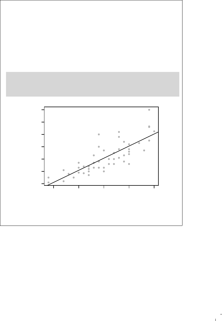
Figure 3.1 is a full example of R code embedded in L
A
T
E
X; we call this
kind of documents Rnw documents hereafter because their filename ex-
tension is Rnw by convention. If we save it as a file minimal.Rnw and
run knit(’minimal.Rnw’) in R as described before, knitr will generate
a L
A
T
E
X output document named minimal.tex. For those who are familiar
with L
A
T
E
X, you can compile this document to PDF via pdflatex. Figure
3.2 is the PDF document compiled from the Rnw document.
What is essential here is how we embedded R code in L
A
T
E
X. In an
Rnw document, <<>>= marks the beginning of code chunks, and @ ter-
minates a code chunk (this description is not rigorous but is often easier

A First Look 13
\documentclass{article}
\begin{document}
\title{A Minimal Example}
\author{Yihui Xie}
\maketitle
We examine the relationship between speed and stopping
distance using a linear regression model:
$Y = \beta_0 + \beta_1 x + \epsilon$.
<<model, fig.width=4, fig.height=3, fig.align='center'>>=
par(mar = c(4, 4, 1, 1), mgp = c(2, 1, 0), cex = 0.8)
plot(cars, pch = 20, col = 'darkgray')
fit <- lm(dist ~ speed, data = cars)
abline(fit, lwd = 2)
@
The slope of a simple linear regression is
\Sexpr{coef(fit)[2]}.
\end{document}
FIGURE 3.1: The source of a minimal Rnw document: see output in
Figure 3.2.
to understand); we have four lines of R code between the two mark-
ers in this example to draw a scatterplot, fit a linear model, and add
a regression line to the scatterplot. The command \Sexpr{} is used to
embed inline R code, e.g., coef(fit)[2] in this example. We can write
chunk options for a code chunk between << and >>=; the chunk options
in this example specified the plot size to be 4 by 3 inches (fig.width and
fig.height), and plots should be aligned in the center (fig.align).
In this minimal example, we have most basic elements of a report:
1. title, author, and date
2. model description
3. data and computation
4. graphics
5. numeric results
All the output is generated dynamically from R. Even if the data has
14 Dynamic Documents with R and knitr
A Minimal Example
Yihui Xie
April 11, 2015
We examine the relationship between speed and stopping distance using a
linear regression model: Y = β
0
+ β
1
x + .
par(mar = c(4, 4, 1, 1), mgp = c(2, 1, 0), cex = 0.8)
plot(cars, pch = 20, col = "darkgray")
fit <- lm(dist ~ speed, data = cars)
abline(fit, lwd = 2)
5 10 15 20 25
0 20 40 60 80 100
speed
dist
The slope of a simple linear regression is 3.9324088.
1
FIGURE 3.2: A minimal example in L
A
T
E
X with an R code chunk, a plot,
and numeric output (regression coefficient).

A First Look 15
---
title: A Minimal Example
---
We examine the relationship between speed and stopping
distance using a linear regression model:
$Y = \beta_0 + \beta_1 x + \epsilon$.
```{r fig.width=4, fig.height=3, fig.align='center'}
par(mar = c(4, 4, 1, 1), mgp = c(2, 1, 0), cex = 0.8)
plot(cars, pch = 20, col = 'darkgray')
fit <- lm(dist ~ speed, data = cars)
abline(fit, lwd = 2)
```
The slope of a simple linear regression is
`r coef(fit)[2]`.
FIGURE 3.3: The source of a minimal Rmd document: see output in
Figure 3.4.
changed, we do not need to redo the report from the ground up, and the
output will be updated accordingly if we update the data and recompile
the report.
3.2.2 An Example in Markdown
L
A
T
E
X may look overwhelming to beginners due to the large number
of commands. By comparison, Markdown (Gruber, 2004) is a much
simpler format. Figure 3.3 is a Markdown example doing the same
analysis with the previous example:
The ideal output from Markdown is an HTML Web page, as shown
in Figure 3.4 (in Mozilla Firefox). Similarly, we can see the syntax for
R code in a Markdown document: ```{r} opens a code chunk, ```
terminates a chunk, and inline R code can be put inside `r `, where `
is a backtick.
A slightly longer example in knitr is a demo named notebook, which
is based on Markdown. It shows not only the potential power of Mark-
down, but also the possibility of building Web applications with knitr.
To watch the demo, run the code below:

16 Dynamic Documents with R and knitr
FIGURE 3.4: A minimal example in Markdown with the same analysis
as in Figure 3.2, but the output is HTML instead of PDF now.

A First Look 17
if (!require("shiny")) install.packages("shiny")
demo("notebook", package = "knitr")
Your default Web browser will be launched to show a Web note-
book. The source code is in the left panel, and the live results are in
the right panel. You are free to experiment with the source code and
recompile the notebook.
3.3 Quick Reporting
If a user only has basic knowledge of R but knows nothing about knitr,
or one does not want to write anything other than an R script, it is also
possible to generate a quick report from this R script using the stitch()
function.
The basic idea of stitch() is that knitr provides a template of the
source document with some default settings, so that the user only needs
to feed this template with an R script (as one code chunk); then knitr
will compile the template to a report. Currently it has built-in templates
for L
A
T
E
X, HTML, and Markdown. The usage is like this:
library(knitr)
stitch("your-script.R")
3.4 Extracting R Code
For a literate programming document, we can either compile it to a re-
port (run the code), or extract the program code in it. They are called
“weaving” and “tangling,” respectively. Apparently the function knit()
is for weaving, and the corresponding tangling function is purl() in
knitr. For example,
library(knitr)
purl("your-file.Rnw")
purl("your-file.Rmd")

18 Dynamic Documents with R and knitr
The result of tangling is an R script; in the above examples, the de-
fault output will be your-file.R, which consists of all code chunks in the
source document.
So far we have been introducing the command line usage of knitr,
and it is often tedious to type the commands repeatedly. In the next
chapter, we show how a decent editor can help edit and compile the
source document with one single mouse click or a keyboard shortcut.

4
Editors
We can write documents for knitr with any text editor, because these
documents are plain text files. For example, lightweight editors like
Notepad under Windows or Gedit under Linux will work. The main
reasons that we need special text editors are
1. we want to input R code chunks more easily, e.g., input <<>>=
and @ with a keyboard shortcut instead of typing these char-
acters every time;
2. we wish to call R and knitr to compile source documents to
PDF/HTML within an editor instead of opening R and typ-
ing the command knitr::knit(), and even better, to send R
code chunks to R from within the editor directly.
There are many mature and nice editors for L
A
T
E
X, HTML, and Mark-
down documents, and some have integrated knitr within them, as we
will explain in the following sections.
4.1 RStudio
RStudio is a relatively new editor specially targeted at R. It may be the
best editor to start with for a beginner, since it has the most compre-
hensive support to Sweave and knitr. RStudio is cross-platform, free
and open-source software; it is available at http://www.rstudio.com.
Besides its excellent support for programming with R, it has a most
notable feature that is missing in many other editors: it has a server
version that looks identical to the desktop version, and we can use R
in a Web browser after we have installed the server version on a Linux
server.
The complete documentation can be found on the website. Here
we only briefly introduce the features related to dynamic documents.
If you are going to write Rnw documents (L
A
T
E
X), the first thing to do
to use knitr in RStudio is to change the option from the menu Tools .
19

20 Dynamic Documents with R and knitr
FIGURE 4.1: Edit an Rnw document in RStudio: there is auto-completion inside the chunk header (we type “fig.”
and will see all candidates); the code chunk can be either inserted from the menu or a keyboard shortcut; the button
Compile PDF supports one-click generation of PDF from Rnw.

Editors 21
Options . Sweave; the default option for weaving (i.e., compiling) Rnw
documents is Sweave, and we can switch it to knitr, as long as we have
installed knitr in R. For more discussion about knitr vs. Sweave, see
Section 16.1. If you plan to work with other types of documents such as
R Markdown, you do not need to configure any options, and RStudio
will give you tips to install the required packages if they are missing.
All document formats supported by RStudio can be found under
the menu File . New. Currently they include R Sweave, R Markdown,
and R HTML. For all document formats, there is one-click compilation
support, i.e., we can click a button to compile a source document to
the corresponding output format (L
A
T
E
X to PDF, Markdown to HTML,
and so on). We can input R code chunks with Ctrl + Alt + I; there
is auto-completion of chunk options in the chunk header; e.g., if we
type “fig.” between << and >>= in an Rnw document, we will see
possible candidates like fig.width, fig.height, and so on. The R code
in chunks can be sent to the R console with Ctrl + Enter, just like what
we do in a normal R script. In this way, we can run certain R code
chunks interactively before we compile a whole document. Figure 4.1
is a screenshot of how an Rnw document looks in RStudio.
For an Rnw document, its final output format is usually PDF (via
L
A
T
E
X). RStudio provides synchronization between the PDF document
and the source document, which implies these features:
1. forward search: we can navigate from one line in the source
document to an appropriate location in the PDF document
that corresponds to the source line;
2. inverse search: we can also click in the PDF document and
RStudio can bring us back to the corresponding lines in the
Rnw source;
3. error navigation: when an error occurs in R or L
A
T
E
X, RStudio
can bring us to a place in the source document that is the
source of the error; this can help us fix problems in R or L
A
T
E
X
code more quickly.
For R Markdown documents, RStudio provides one-click compilation
to a variety of formats, including HTML. Besides, it can also base64 en-
code images and render L
A
T
E
X math expressions (through the MathJax
library) in the HTML output. The former feature is to guarantee that
the HTML page generated is self-contained, i.e., it does not depend on
external images since they have been embedded in the page; the lat-
ter feature is especially useful for statisticians when they want to write
math in a Web page.
The R Markdown (Rmd) format is fairly simple, and can be easily
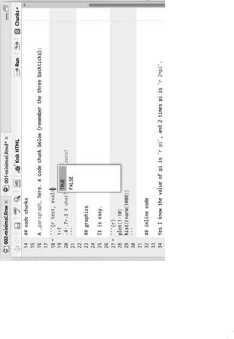
22 Dynamic Documents with R and knitr
FIGURE 4.2: Edit an Rmd document in RStudio: there is also auto-completion for chunk option values; the button Knit
HTML supports one-click generation of an HTML page from Rmd.

Editors 23
mastered in five minutes. Due to its simplicity, there has been a huge
number of reports written in this format and published on RPubs, a
free platform provided by RStudio to host knitr reports from users. See
http://rpubs.com for more examples. Figure 4.2 shows a sample Rmd
document in RStudio.
We mentioned quick reporting in Section 3.3, and this is also sup-
ported in RStudio. For an R script in RStudio, we can create an “R
Notebook” (a report purely based on an R script) from it by clicking the
button on the toolbar.
4.2 L
Y
X
L
Y
X is essentially a front-end for L
A
T
E
X, which has a nice GUI to assist
document writing. On screen, it looks like many word processors, but
at its core, it is L
A
T
E
X. One major difference between raw L
A
T
E
X edi-
tors and L
Y
X is that we only see \alpha + \beta in raw L
A
T
E
X, whereas
we see α + β in L
Y
X, which is essentially \alpha + \beta behind the
screen. Everything is L
A
T
E
X in L
Y
X but our vision is not distorted by a
full screen of backslashes.
Since version 2.0.3, L
Y
X has started to support knitr as an official
module. Details can be found at http://yihui.name/knitr/demo/lyx/.
This module works in this way:
∗.lyx
LyX
−→ ∗.Rnw
R+knitr
−→
(
∗.tex
LaTeX
−→ ∗.pd f (weave)
∗.R (tangle)
Note that currently Rnw is the only possible format to use in L
Y
X. It
seems we are mixing R code with L
Y
X, but L
Y
X is really only a wrapper
so we are actually embedding R code in Rnw documents.
For Linux and Mac OS users, the usage of the module is:
1. create a new L
Y
X document;
2. go to Document . Settings . Modules and insert the module named
Rnw (knitr);
3. insert R code chunks into the document with Insert . T
E
X Code,
then start typing <<>>= and @ as usual.
Click the View button on the toolbar or press Ctrl + R to compile the
document to PDF and view the results. We can also extract R code from
a L
Y
X document from the menu File . Export . R/S code. A screenshot
of L
Y
X with R code is shown in Figure 4.3.
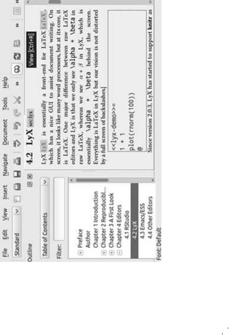
24 Dynamic Documents with R and knitr
FIGURE 4.3: Using knitr in L
Y
X: R code is inserted in a red box using the Rnw syntax; when we click the View button,
we will see a PDF document compiled through knitr and L
Y
X.

Editors 25
There is one more step before we can use the knitr module under
Windows: go to Tools . Preferences . Paths . PATH prefix and add the bin
path of R there, which is often like C:\Program Files\R\R-x.x.x\bin and
you can find it in R:
R.home("bin")
After you have made this change, you need to reconfigure L
Y
X by
Tools . Reconfigure. This is to make sure L
Y
X knows where R is installed
so that it can call R and knitr to compile the Rnw document. Specifi-
cally, it needs to know where Rscript.exe is. If it is not present in PATH,
the knitr module will be unavailable. This step is often not needed for
Linux and Mac OS because these systems will put the R executable on
PATH by default.
Although the graphical interface looks easy enough to use, we still
strongly recommend users to master L
A
T
E
X before trying L
Y
X; otherwise
it can be difficult to diagnose L
A
T
E
X problems when errors occur. L
Y
X is
not Word, after all.
4.3 Emacs/ESS
ESS (Emacs Speaks Statistics) is an add-on package for the text editor
Emacs (Rossini et al., 2004). It supports statistical software packages
like R, S-Plus, SAS, JAGS, and so on. The support for knitr was added
after version 12.09; before that, only Sweave was supported.
ESS is also free and open-source software; it is available at http:
//ess.r-project.org. After it has been installed along with Emacs, it
is fairly easy to call knitr in Emacs. The default option for Rnw doc-
uments is Sweave, and we can change it to knitr with the following
commands (in Emacs key notation, M stands for the Meta key, which is
the Alt key on most keyboards, and M-x means to hold Meta and press
x):
M-x customize-group
ess-R
Find the ess-swv-processor option and change it to knitr. Then we can
create a new Rnw document, press M-n s to compile Rnw to T
E
X, and
M-n P to compile T
E
X to PDF.
The support of Rmd documents and other document formats in ESS
is still under development. According to the developers, this feature

26 Dynamic Documents with R and knitr
may come in ESS 13.03, and readers can pay attention to their official
announcement in the future.
4.4 Other Editors
It is not hard to add support in other editors as long as they allow defin-
ing custom commands to compile documents. Generally speaking, the
custom command looks like:
Rscript -e "library(knitr); knit('input.ext')"
This command calls R to load the knitr package and compile the
input document named input.ext using the function knit().
WinEdt (proprietary software) has a mode named R-Sweave to sup-
port knitr; and Tinn-R (free) has built-in support. It is also possible
to configure other text editors such as Texmaker, Eclipse, TextMate,
T
E
XShop, and Vim so that we can conveniently compile reports inside
them. The configuration instructions are collected at http://yihui.
name/knitr/demo/editors/.

5
Document Formats
The design of the knitr package is flexible enough to process any plain
text documents in theory. Below are the three key components of the
design:
1. a source parser
2. a code evaluator
3. an output renderer
The parser parses the source document and identifies computer code
chunks as well as inline code from the document; the evaluator exe-
cutes the code and returns results; the renderer formats the results from
computing in an appropriate format, which will finally be combined
with the original documentation.
The code evaluator is independent of the document format, whereas
the parser and the renderer have to take the document format into con-
sideration. The former corresponds to the input syntax, and the latter
is related to the output syntax.
5.1 Input Syntax
Regular expressions (Friedl, 2006, or see Wikipedia) are used to identify
code blocks (chunks) and other elements such as inline code in a docu-
ment. These regular expression patterns are stored in the all_patterns
object in knitr. For example, the pattern for the beginning of a code
chunk in an Rnw document is:
all_patterns$rnw$chunk.begin
## [1] "^\\s*<<(.*)>>=.*$"
In a regular expression, ^ means the beginning of a character string;
\s* matches any number (including zero) of white spaces; .* matches
27

28 Dynamic Documents with R and knitr
any number of any characters. This regular expression means “any
white spaces in the beginning of the line + << + any characters + >>=,”
therefore the lines below are possible chunk headers:
<<>>=
<<foo>>=
<<bar, echo=TRUE>>=
<<a=1, b=2>>=
And these are not valid chunk headers (<< does not appear in the
beginning of the line in the first one; there is only one > in the second
one; = is missing in the third one):
hi<<>>=
<<foo>=
<<bar>>
Two more technical notes about the regular expression above:
1. \s denotes a white space in regular expressions, but in R we
have to write double backslashes because \\ in an R string re-
ally means one backslash (the first backslash acts as escaping
the second character, which is also a backslash); the backslash
as the escape character can be rather confusing to beginners,
and the rule of thumb is, when you want a real backslash,
you may need two backslashes;
2. the braces () in the regular expression group a series of char-
acters so that we can extract them with back references, e.g.,
we extract the second group of characters from abbbc:
# [b]+ means to match 'b' for one or more times
gsub("(a)([b]+)(c)", "\\2", "abbbc")
## [1] "bbb"
We need to extract the chunk options in the chunk headers,
and that is why we wrapped .* in () in the regular expres-
sion as <<(.*)>>=.
5.1.1 Chunk Options
As mentioned in Chapter 3, we can write chunk options in the chunk
header. The syntax for chunk options is almost exactly the same as the

Document Formats 29
syntax for function arguments in R. They are of the form
option = value
There is nothing to remember about this syntax due to the consis-
tency with the syntax of R: as long as the option values are valid R
code, they are valid to knitr. Besides constant values like echo = TRUE
(a logical value) or out.width = ’\\linewidth’ (character string) or
fig.height = 5 (a number), we can write arbitrary valid R code for
chunk options, which makes a source document programmable. Here
is a trivial example:
<<foo, eval=if (bar < 5) TRUE else FALSE>>=
Suppose bar is a numeric variable created in the source document
before this chunk. We can pass an expression if (bar < 5) TRUE else
FALSE to the option eval, which makes the option eval depend on the
value of bar, and the consequence is we evaluate this chunk based on
the value of bar (if it is greater than 5, the chunk will not be evaluated),
i.e., we are able to selectively evaluate certain chunks. This example is
supposed to show that we can write arbitrarily complicated R expres-
sions in chunk options. In fact, it can be simplified to eval = bar <
5 since the expression bar < 5 normally returns TRUE or FALSE (unless
bar is NA).
5.1.2 Chunk Label
The only possible exception is the chunk label, which does not have to
follow the syntax rule. In other words, it can be invalid R code. This is
due to both historical reasons (Sweave convention) and laziness (avoid
typing quotes). Strictly speaking, the chunk label, as a part of chunk
options, should take a character value, hence it should be quoted, but
in most cases, knitr can take care of the unquoted labels and quote them
internally, even if the “objects” used in the label expression do not exist.
Below are all valid ways to write chunk labels:
<<foo>>=
<<foo-bar>>=
<<foo_bar>>=
<<"foo">>=
<<'foo-bar'>>=
<<label="foo">>=
<<echo=FALSE, label="foo-bar">>=

30 Dynamic Documents with R and knitr
Chunk labels are supposed to be unique id’s in a document, and
they are mainly used to generate external files such as images (Chapter
7) and cache files (Chapter 8). If two non-empty chunks have the same
label, knitr will stop and emit an error message, because there is poten-
tial danger that the files generated from one chunk may override the
other chunk. If we leave a chunk label empty, knitr will automatically
generate a label of the form unnamed-chunk-i, where i is an incremen-
tal chunk number from 1, 2, 3, ···.
5.1.3 Global Options
Chunk options control every aspect of a code chunk, as we will see in
more detail in Chapters 6 through 11. If there are certain options that
are used commonly for most chunks, we can set them as global chunk
options using the object opts_chunk. Global options are shared across
all the following chunks after the location in which the options are set,
and local options in the chunk header can override global options. For
example, we set the option echo to FALSE globally:
opts_chunk$set(echo = FALSE)
Then for the two chunks below, echo will be FALSE and TRUE, re-
spectively:
<<foo>>=
1+1
@
<<bar, echo=TRUE>>=
rnorm(10)
@
5.1.4 Chunk Syntax
The original syntax of literate programming is actually this: use one
marker to denote the beginning of computer code (<<>>=), and one
marker to denote the beginning of the documentation (@). This has a
subtle difference from what we introduced in Chapter 3. In the literate
programming paradigm, this is what a source document may look like:
@
This is documentation.
@

Document Formats 31
Another line of documentation.
<<>>=
1 + 1 # some code
<<>>=
rnorm(10) # another code chunk
@
More documentation.
In knitr syntax, we open and close code chunks instead of opening
code chunks and opening documentation chunks. The reason why we
dropped the traditional syntax is that in a report, the code chunks often
appear less frequently than normal text, so we only focus on the syntax
for code chunks. It also looks more intuitive that we are “embedding”
code into a report. Based on the new syntax, this is also a legitimate
fragment of a source document for knitr:
Documentation here.
<<>>=
1+1
<<>>=
rnorm(10)
@
More documentation.
5.2 Document Formats
We have been using the syntax of Rnw documents as examples. Next
we are going to introduce how to write R code in other document for-
mats; Table 5.1 is a summary of the syntax. Note that code chunks can
be indented by any number of spaces in all document formats.
5.2.1 Markdown
For an R Markdown (Rmd) document, we write code chunks between
```{r} and ```, and inline R code is written in `r `. Chunk options
are written before the closing brace in the chunk header. Note that the
inline R code is not allowed to contain backticks, e.g., `r pi*2` is fine,
but `r `pi`*2` is not; although `pi`*2 is valid R code, the parser is
unable to know the first backtick is not for terminating the inline R code
expression.

32 Dynamic Documents with R and knitr
TABLE 5.1: A syntax summary of all document formats: R L
A
T
E
X, R Markdown, R HTML, R reStructuredText, R
AsciiDoc, R Textile, and brew.
format start end inline
Rnw <<*>>= @ \Sexpr{x}
Rmd ```{r *} ``` `r x`
Rhtml <!--begin.rcode * end.rcode--> <!--rinline x-->
Rrst .. {r *} .. .. :r:`x`
Rtex % begin.rcode * % end.rcode \rinline{x}
Rasciidoc // begin.rcode * // end.rcode `r x`
Rtextile ###. begin.rcode * ###. end.rcode @r x@
brew <% x %>

Document Formats 33
Markdown allows us to write using an easy-to-read, easy-to-write
plain text format, then convert it to structurally valid XHTML or HTML.
As long as one knows how to write emails, one can learn it in a few
minutes: http://en.wikipedia.org/wiki/Markdown. Below is a short
example:
# First level header
## Second level
This is a paragraph. This is **bold**, and _italic_.
- list item
- list item
Backticks produce the `<code>` tag. This is [a link](url),
and this is an . A block of code (`<pre>` tag):
1 + 1
rnorm(10)
### Third level section title
You can write an ordered list:
1. item 1
2. item 2
The original Markdown syntax was designed to be simple, so it is
inevitable to have some restrictions in terms of an authoring environ-
ment, such as the ability to write tables, L
A
T
E
X math expressions, or,
bibliography. In some cases, such as writing a short homework assign-
ment, we do not need complicated features, so Markdown should work
reasonably well.
One problem of Markdown is its derivatives: there are a number of
variants such as Pandoc’s Markdown (http://johnmacfarlane.net/
pandoc), Github Flavored Markdown (http://github.com), kramdown
(http://kramdown.rubyforge.org) and so on. These flavors may have
their own definitions of how to write certain elements (such as tables).
CommonMark (http://commonmark.org) is an effort at defining the
Markdown syntax unambiguously, and Pandoc’s Markdown is com-
patible with the CommonMark standards. Besides, Pandoc is probably
the most comprehensive tool for Markdown at the moment. It added
many useful extensions to the original Markdown such as:

34 Dynamic Documents with R and knitr
1. Fenced code blocks within a pair of three backticks;
2. L
A
T
E
X math via either plain L
A
T
E
X (for PDF output) or MathJax
(http://mathjax.org, for HTML output), which allows us
to write math equations in Web pages using the L
A
T
E
X syntax,
i.e., $math$ or $$math$$;
3. Metadata for the document, e.g., the title, author, and date
information;
4. Tables, with columns separated by white spaces or pipes;
5. Definition lists, footnotes, and citations, etc.
Below is how some of the extensions look:
---
title: The Title of My Report
author: Yihui Xie
---
Write code under ``` or indent by 4 spaces as usual.
```r
1 + 1
rnorm(10)
```
Inline math: $\alpha + \beta$. Display style:
$$f(x) = x^{2} + 1$$
A simple table from the citation [@joe2014]:
| id | age | sex |
|:----|----:|:---:|
| a | 49 | M |
| b | 32 | F |
More importantly, Pandoc can convert Markdown to several other
document formats, including PDF/L
A
T
E
X, HTML, Word (Microsoft Word
or OpenOffice), and presentation slides (either L
A
T
E
X beamer or HTML5
slides). The R package rmarkdown (Allaire et al., 2015a) is based on
knitr and Pandoc, and contains a few commonly used output formats
so users can quickly create reasonably beautiful output by default.
The rmarkdown package was introduced by the RStudio develop-
ers, so it is not surprising that the R Markdown document format is

Document Formats 35
best supported by RStudio. When we open or create an Rmd document
in RStudio (File . New . R Markdown), we can see a wizard asking you
which output format you want. We will cover R Markdown in detail in
Chapter 14.
5.2.2 L
A
T
E
X
Markdown was primarily designed for the Web, and for more compli-
cated typesetting purposes, L
A
T
E
X may be preferred. For example, this
book was written in L
A
T
E
X. Oetiker et al. (1995) is a classic tutorial for
beginners to learn L
A
T
E
X. The learning curve can be steep but it is re-
warding if you care a lot about typesetting by yourself.
For L
A
T
E
X documents, R code chunks are embedded between <<>>=
and @, and inline R code is written in \Sexpr{}, as we have seen many
times before.
5.2.3 HTML
HTML (Hyper-Text Markup Language) is the language behind Web
pages; normally we do not see HTML code directly because the Web
browser has parsed it and rendered the elements. For example, when
we see bold texts, the source code might be <strong>bold</strong>.
Most Web browsers can show the HTML source code; e.g., for Firefox
and Google Chrome, we can press Ctrl + U to view the page source.
There is a large (but limited) number of tags in HTML to represent
different elements in a page. HTML is like L
A
T
E
X in the sense that we
can have precise control over the typesetting by carefully organizing
the tags/commands. The price to pay is that it may take a long time
to write a document since there are many tags to type. That is why
Markdown can be better for small-scale documents. Anyway, due to
the fact that HTML has the full power, sometimes we have to use it.
Below is an example of an HTML document:
<html>
<head>
<title>This is an HTML page</title>
</head>
<body>
<p>This is a <em>paragraph</em>.</p>
<div>A <code>div</code> layer.</div>
<!-- I'm a comment; you cannot see me. -->
</body>
</html>

36 Dynamic Documents with R and knitr
To write R code in an HTML document, we use the comment syntax
of HTML, e.g.,
<!--begin.rcode test-html, eval=TRUE
1 + 1
rnorm(10)
end.rcode-->
<p>And here is the value of pi: <!--rinline pi -->.</p>
5.2.4 reStructuredText
We can also embed R code in a reStructuredText (reST) document (http:
//docutils.sourceforge.net/rst.html), which is like Markdown but
more powerful (and complicated accordingly). Below is an example of
R code embedded in an R reST document:
A reST document for knitr
=========================
This is a reStructuredText document (*.Rrst). Here is how
we write R code for **knitr**:
.. {r test-rst, eval=TRUE}
1 + 1
rnorm(10)
.. ..
The value of pi is :r:`pi`.
The Docutils system (written in Python) is often used to convert
reST documents to HTML.
5.2.5 AsciiDoc
AsciiDoc (http://en.wikipedia.org/wiki/AsciiDoc) is a plain-text
document format that can be converted to multiple types of output,
such as software documentation, articles, books, and HTML pages. Be-
low is a minimal R AsciiDoc example for writing a book:
= The Book Title
:author: A Knitter

Document Formats 37
== The first chapter
Hello world!
// begin.rcode test, eval=TRUE
1 + 1
rnorm(10)
// end.rcode
The value of pi is `r pi`.
5.2.6 Textile
Textile is yet another lightweight markup language, and it is usually
converted to HTML. You can find more information on the Wikipedia
page http://en.wikipedia.org/wiki/Textile_(markup_language).
Here is an R Textile example demonstrating the syntax:
h1. Knitting Textile Files
Hello world!
###. begin.rcode test, tidy=FALSE
if (1 + 1 == 2) {
'of course!'
}
###. end.rcode
And an inline expression @r 2*pi@.
5.2.7 Customization
It is possible to define one’s own syntax to parse a source document. As
we have seen before, the parsing is done through regular expressions.
Internally, knitr uses the object knit_patterns to manage the regular
expressions. For example, the three major patterns for this book are:
knit_patterns$get(
c("chunk.begin", "chunk.end", "inline.code")
)

38 Dynamic Documents with R and knitr
## $chunk.begin
## [1] "^\\s*<<(.*)>>=.*$"
##
## $chunk.end
## [1] "^\\s*@\\s*(%+.*|)$"
##
## $inline.code
## [1] "\\\\Sexpr\\{([^}]+)\\}"
To specify our own syntax, we can use knit_patterns$set(), which
will override the default syntax, e.g.,
knit_patterns$set(
chunk.begin = "^<<r(.*)", chunk.end = "^r>>$",
inline.code = "\\{\\{([^}]+)\\}\\}"
)
Then we will be able to parse a document like this with the custom
syntax:
<<r test-syntax, eval=TRUE
1 + 1
x <- rnorm(10)
r>>
The mean of x is {{mean(x)}}.
In practice, however, this kind of customization is often unneces-
sary. It is better to follow the default syntax, otherwise additional in-
structions will be required in order to compile a source document.
There is a series of functions with the prefix pat_ in knitr, which
are convenience functions to set up the syntax patterns, e.g., pat_rnw()
calls knit_hooks$set() to set patterns for Rnw documents. All pattern
functions include:
grep("^pat_", ls("package:knitr"), value = TRUE)
## [1] "pat_asciidoc" "pat_brew" "pat_html"
## [4] "pat_md" "pat_rnw" "pat_rst"
## [7] "pat_tex" "pat_textile"
When parsing a source document, knitr will first decide which pat-
tern list to use according to the filename extension; e.g., *.Rmd docu-
ments use the R Markdown syntax. If the file extension is unknown,

Document Formats 39
knitr will further detect the code chunks in the document and see if the
syntax matches with any existing pattern list; if it does, that pattern list
will be used; e.g., for a file foo.txt, the extension txt is unknown to knitr,
but if this file contains a code chunk that begins with ```{r}, knitr will
use the R Markdown syntax automatically.
5.3 Output Renderers
The evaluate package (Wickham, 2015) is used to execute code chunks,
and the eval() function in base R is used to execute inline R code. The
latter is easy to understand and made possible by the power of “com-
puting on the language” (R Core Team, 2014) of R. Suppose we have a
code fragment 1+1 as a character string; we can parse and evaluate it as
R code:
eval(parse(text = "1+1"))
## [1] 2
For code chunks, it is more complicated. The evaluate package takes
a piece of R source code, evaluates it, and returns a list containing re-
sults of six possible classes: character (normal text output), source
(source code), warning, message, error, and recordedplot (plots).
In order to write these results into the output, we have to take the
output format into consideration. For example, if the source code is
1+1 and the output format is T
E
X, we may use the verbatim environ-
ment, whereas if the output is supposed to be HTML, we may write
<pre>1+1</pre> into the output instead. The key question is, how
should we wrap up the raw results from R? This is answered by the
knit_hooks object, which contains a list of output hook functions to
construct the final output. A hook function is often defined in this form:
hook_fun <- function(x, options) {
# returns a character string with markup
}
In an output hook, x is usually the raw output from R, and options
is a list of current chunk options. The hook names in knit_hooks cor-
responding to the output classes are listed in Table 5.2.
If we want to put the message output (emitted from message() func-

40 Dynamic Documents with R and knitr
TABLE 5.2: Output hook functions and the object classes of results from
the evaluate package.
Class Output hook Arguments
source source x, options
character output x, options
recordedplot plot x, options
message message x, options
warning warning x, options
error error x, options
chunk x, options
inline x
text x
document x
tion) into a custom L
A
T
E
X environment, say, Rmessage, we can set the
message hook as:
knit_hooks$set(message = function(x, options) {
paste0("\\begin{Rmessage}\n", x, "\\end{Rmessage}")
})
Of course, we have to define the Rmessage environment in advance
in the L
A
T
E
X preamble, e.g.,
\newenvironment{Rmessage}{
\rule[0.5ex]{1\columnwidth}{1pt} % a horizontal line
}{
\rule[0.5ex]{1\columnwidth}{1pt}
}
Then, whenever we have a message in the output, we will see a
horizontal line above and below it.
By default, knitr will set up a series of default output hooks for each
output format, so normally we do not have to set up all the hooks by
ourselves. A series of functions with the prefix render_ in knitr can be
used to set up default output hooks for various output formats:
grep("^render_", ls("package:knitr"), value = TRUE)
## [1] "render_asciidoc" "render_html"
## [3] "render_jekyll" "render_latex"
## [5] "render_listings" "render_markdown"
## [7] "render_rst" "render_sweave"
## [9] "render_textile"

Document Formats 41
This is all you need to do if you want to go back to the Sweave style:
The quick brown fox jumps over the lazy dog the quick brown fox jumps
over the lazy dog the quick brown fox jumps over the lazy dog.
> 1 + 1
[1] 2
> rnorm(30)
[1] -0.56048 -0.23018 1.55871 0.07051 0.12929 1.71506 0.46092
[8] -1.26506 -0.68685 -0.44566 1.22408 0.35981 0.40077 0.11068
[15] -0.55584 1.78691 0.49785 -1.96662 0.70136 -0.47279 -1.06782
[22] -0.21797 -1.02600 -0.72889 -0.62504 -1.68669 0.83779 0.15337
[29] -1.13814 1.25381
The quick brown fox jumps over the lazy dog the quick brown fox jumps
over the lazy dog the quick brown fox jumps over the lazy dog.
1
FIGURE 5.1: The Sweave style in knitr: if we run render_sweave() in the
beginning of an Rnw document, we will see the Sweave style.
The functions render_latex(), render_html(), and render_markdown() are
called when the output formats are L
A
T
E
X, HTML, and Markdown, re-
spectively; render_sweave() and render_listings() are two variants of L
A
T
E
X
output — the former uses the traditional Sweave environments defined
in Sweave.sty (e.g., Sinput and Soutput, etc.), and the latter uses the list-
ings package in L
A
T
E
X to decorate the output. See Figure 5.1 and Figure
5.2 for how the two styles look.
Note that if we want to set up the output hooks, it is better to do
it in the very beginning of a source document so that the rest of the
output can be affected. For example, the chunk below can be the first
chunk of an Rnw document (the chunk option include = FALSE means
do not show anything from this chunk in the output because it is not
interesting to the readers):
<<setup, include=FALSE>>=
render_sweave()
@
Then the output will be rendered in the Sweave style. This book
used the default L
A
T
E
X style, which supports syntax highlighting, and
code chunks are put in gray shaded boxes.
Among all output hooks in Table 5.2, there are five special hooks
that need further explanation:

42 Dynamic Documents with R and knitr
This is all you need to do if you want to use the listings package:
The quick brown fox jumps over the lazy dog the quick brown fox jumps
ove r the lazy dog the quick brown fox jumps over the lazy dog.
1 + 1
[1] 2
rnorm ( 3 0)
[1] -0.56 048 -0.230 18 1.558 71 0 .070 51 0.1 2929 1.71 506 0 .460 92
[8] -1.26 506 -0.686 85 - 0.44566 1 .224 08 0.35 981 0.40 077 0 .110 68
[15] -0 .55584 1.78 691 0 .497 85 -1.96 662 0.701 36 -0 .47 279 -1.067 82
[22] -0 .21797 -1. 02600 -0.72889 -0.62504 -1. 68669 0.83 779 0.153 37
[29] -1 .13814 1.25 381
The quick brown fox jumps over the lazy dog the quick brown fox jumps
ove r the lazy dog the quick brown fox jumps over the lazy dog.
1
FIGURE 5.2: The listings style in knitr: render_listings() produces a style
like this (colored text and gray shading).
• the plot hook takes the filename as input x which is a character string
of the filename (e.g., foo.pdf); below is a simplified version of the plot
hook for L
A
T
E
X output (the actual hook is much more complicated than
this, because there are many chunk options to take into account, such
as out.width and out.height, etc.)
knit_hooks$set(plot = function(x, options) {
paste("\\includegraphics{", x, "}", sep = "")
})
• the chunk hook takes the output of the whole chunk as input, which
is generated from other hooks such as source, output, and message,
etc.; for example, if we want to put the chunk output in a div tag with
the class Rchunk in HTML, we can define the chunk hook as:
knit_hooks$set(chunk = function(x, options) {
paste("<div class='Rchunk'>", x, "</div>")
})
then we need to define the style of Rchunk in the CSS stylesheet for
this HTML document;
• the inline hook is not associated with a code chunk; it defines how
to format the output from inline R code. For example, we may want

Document Formats 43
to round all the numbers from inline output to 2 digits and we can
define the inline hook as:
knit_hooks$set(inline = function(x) {
if (is.numeric(x))
x <- round(x, 2)
as.character(x) # convert x to character and return
})
knitr takes care of rounding in the default inline hook (Section 6.1), so
we do not really have to reset this hook;
• the text hook processes text chunks, i.e., narratives; for example, we
set up a hook to trim the white spaces around the text chunks:
knit_hooks$set(text = function(x) {
gsub("^\\s*|\\s*$", "", x)
})
• the document hook is similar to the chunk hook, and it takes the output
of the whole document as input x; this hook can be useful for post-
processing the document; in fact, this book used this hook to add a
vertical space \medskip{} under all table captions (before the tabular
environment):
knit_hooks$set(document = function(x) {
gsub("\\begin{tabular}", "\\medskip{}\\begin{tabular}",
x, fixed = TRUE)
})
5.4 R Scripts
There is a special source document format in knitr, which is essentially
an R script with roxygen comments (for more on roxygen, see Wickham
et al. (2015) and Appendix A.1). We know a normal R comment starts
with #, and a roxygen comment has an apostrophe after #, e.g.,

44 Dynamic Documents with R and knitr
#' this is a roxygen comment
##' me too
Sometimes we do not want to mix R code with normal text, but write
text in comments, so that the whole document is a valid R script. The
function spin() in knitr can deal with such R scripts if the comments
are written using the roxygen syntax. The basic idea of spin() is also
inspired by literate programming: when we compile this R script, #'
will be removed so that normal text is “restored,” and R code will be
evaluated. Anything that is not behind a roxygen comment is treated
as a code chunk. To write chunk options, we can use another type of
special comment #+ or #- followed by chunk options. Below is a simple
example:
#' Introduce the method here; then write R code:
1 + 1
x <- rnorm(10)
#' It is also possible to write chunk options, e.g.,
#'
#+ test-label, fig.height=4
plot(x)
#' The document is done now.
We can save this script to a file called test.R, and compile it to a
report:
library(knitr)
spin("test.R")
The spin() function has a format argument that specifies the output
document format (default to R Markdown). For example, if format =
’Rnw’, the R code will first be inserted between <<>>= and @, and then
compiled to generate L
A
T
E
X output.
This looks similar to the stitch() function in Section 3.3, which also
creates a report based on an R script, but spin() makes it possible to
write text chunks and stitch() can only use a predefined template, so
there is less freedom.

6
Text Output
From this chapter forward, we will start touching on the chunk op-
tions in knitr. First, in this chapter, we explain how to tune text output,
including output from inline R code as well as text output from code
chunks.
6.1 Inline Output
If the inline R code produces character results, they will be directly writ-
ten into the output. When the result is numeric, scientific notation will
be considered to denote the numbers that are too big or too small.
The threshold between scientific notation and fixed notation is the
R option scipen (see ?options for details). By default (scipen = 0), if
a positive number is bigger than 10
4
or smaller than 10
−4
(this applies
to the absolute values of negative numbers too), it will be denoted in
scientific notation. Depending on the output format (L
A
T
E
X or HTML),
knitr will use the appropriate code, such as $3.14 \times 10^5$ or
3.14 × 10<sup>5</sup>. The reason for scientific notation is to
make it easier to read numbers such as small P-values, e.g., compare
0.000143 with 1.43 ×10
−4
.
Another R option digits controls how many digits a number should
be rounded to. R’s default is 7, which often makes a number unnec-
essarily “precise.” We can change the defaults in the first chunk of a
document, like:
# numbers >= 10^5 will be denoted in scientific
# notation, and rounded to 2 digits
options(scipen = 1, digits = 2)
For example, this book uses digits = 4, and a number 123456789
will become 1.2346 × 10
8
after the book source is compiled to PDF.
Note that these two options are not specific to knitr; they are global
45

46 Dynamic Documents with R and knitr
options in R. If we are not satisfied with the default inline output, we
can rewrite the inline hook as introduced in Section 5.3. Next we are
going to introduce chunk options that affect the text output from code
chunks.
For character results, we may have to take care of some special char-
acters especially for L
A
T
E
X and HTML, e.g., % means comments in L
A
T
E
X,
and a literal ampersand (&) has to be written as & in HTML. See
Section 12.3.6 for how to escape these characters if needed.
In most cases, characters are written as is in the output. For example,
\Sexpr{letters[1]} produces “a” in the output of an Rnw document,
and `r month.name[2]` in an Rmd document produces “February”. A
special case is the R HTML document: inline character results are writ-
ten in the <code></code> tag by default, e.g., <!--rinline 'ABC'-->
produces <code class=’knitr inline’>ABC</code>. To get rid of the
code tag, we can wrap the results in the function I(), which means to
print the characters as is, e.g., <!--rinline I('ABC')-->.
6.2 Chunk Output
The “text output” in this section refers to any output from R that is not
graphics, so even messages and warnings are classified as text output.
6.2.1 Chunk Evaluation
The chunk option eval (TRUE or FALSE) decides whether a code chunk
should be evaluated. When a chunk is not evaluated, there will be no
results returned except the original source code. This option can also
take a numeric vector to specify which expressions are to be evaluated;
in this case, the code that is set not to be evaluated will be commented
out. For the chunk below, we set eval = -2, which means the second
expression will not be evaluated:
1 + 1
## [1] 2
## if (TRUE) {
## print("hi")
## }
dnorm(0)
## [1] 0.3989

Text Output 47
6.2.2 Code Formatting
The function tidy_source() in the formatR package (Xie, 2015a) will be
used to reformat R code (when the chunk option tidy = TRUE), e.g., it
can add spaces and indentation, break long lines into shorter ones, and
automatically replace the assignment operator = to <-; see the manual
of formatR for details. The chunk option tidy.opts (a list) is passed
to tidy_source() to control the formatting of R code. The example below
shows the effect of tidy = TRUE/FALSE:
# option tidy=FALSE
for(k in 1:10){j=cos(sin(k)*k^2)+3;print(j-5)}
# option tidy=TRUE
for (k in 1:10) {
j <- cos(sin(k) * k^2) + 3
print(j - 5)
}
We can pass an argument width.cutoff to tidy_source() through
the chunk option tidy.opts = list(width.cutoff = 40) so that the
width of source code is roughly 40, e.g.,
0 + 1 + 2 + 3 + 4 + 5 + 6 + 7 + 8 + 9 + 0 +
1 + 2 + 3 + 4 + 5 + 6 + 7 + 8 + 9 + 0 +
1 + 2 + 3 + 4 + 5 + 6 + 7 + 8 + 9 + 0 +
1 + 2 + 3 + 4 + 5 + 6 + 7 + 8 + 9
## [1] 180
# all arguments of tidy_source()
names(formals(formatR::tidy_source))
## [1] "source" "comment" "blank"
## [4] "arrow" "brace.newline" "indent"
## [7] "output" "text" "width.cutoff"
## [10] "..."
6.2.3 Code Decoration
Syntax highlighting comes by default in knitr (chunk option highlight
= TRUE), since it enhances the readability of the source code — charac-
ter strings, comments, and function names, etc., are in different colors.

48 Dynamic Documents with R and knitr
This is achieved by the highr package (Qiu and Xie, 2015). This op-
tion only works for L
A
T
E
X and HTML output, and it is not necessary for
Markdown because there are other libraries that can highlight code in
Web pages; e.g., the JavaScript library highlight.js is widely used to do
syntax highlighting for HTML pages.
For L
A
T
E
X output, the L
A
T
E
X package framed is used to decorate code
chunks with a light gray background (as we can see in this book). If this
package is not found in the system, a version will be copied directly
from knitr. The output for HTML documents is styled with CSS, which
looks similar to L
A
T
E
X (with gray shadings and syntax highlighting).
The background color is controlled by the chunk option background,
which takes a color value such as ’#FF0000’, ’red’, or rgb(1, 0, 0)
(as long as it is a valid color in R).
The prompt characters are removed by default because they mangle
the R source code in the output and make it difficult to copy R code. The
R output is masked in comments by default based on the same rationale
(option comment = ’##’). In fact, this was largely motivated from the
author’s experience of grading homework when he was a teaching as-
sistant; with the default prompts, it is difficult to verify the results in the
homework, because it is so inconvenient to copy the source code. Any-
way, it is easy to revert to the output with prompts (set option prompt
= TRUE), and we will quickly realize the inconvenience to the readers
if they want to run the code in the output document, e.g., the chunk
below uses prompt = TRUE and comment = NA:
> x <- rnorm(5)
> x
[1] -0.01156 -0.90915 0.37367 1.90694 0.16459
> var(x)
[1] 1.041
While this may seem to be irrelevant to reproducible research, we
would argue that it is of great importance to design styles that look ap-
pealing and helpful at first glance, which can encourage users to write
reports in this way.
For L
A
T
E
X output, we can also specify the font size of the chunk out-
put via the size option, which takes the value of L
A
T
E
X font sizes such
as footnotesize, small, large, and Large, etc., (the default size is normal-
size). It is helpful to set a smaller font size when the output is long and
the space is limited, e.g., in beamer slides. The chunk below uses size
= ’footnotesize’:

Text Output 49
<<font-size, size='footnotesize'>>=
x <- rnorm(20, mean = 5, sd = 3)
x^2
## [1] 5.039 8.314 10.604 5.749 28.855 38.501 14.089
## [8] 10.535 16.023 94.736 32.549 33.854 37.890 54.440
## [15] 41.333 31.910 8.445 2.227 46.454 25.077
@
6.2.4 Show/Hide Output
We can show or hide different parts of the text output including the
source code, normal text output, warnings, messages, errors, and the
whole chunk. Below are the corresponding chunk options with default
values in the braces:
echo (TRUE) whether to show the source code; it can also take a numeric
vector like the eval option to select which expressions to show in the
output, e.g., echo = 1:3 selects the first 3 expressions, and echo = -5
means do not show the 5th expression.
results (’markup’) how to wrap up the normal text output that would
have been printed in the R console if we had run the code in R; the
default value means to mark up the results in special environments
such as L
A
T
E
X environments or HTML div tags; other possible values
are:
’asis’ write the raw output from R to the output document without
any markups, e.g., the source code cat(’<em>emphasize</em>’)
can produce an italic text in HTML when results = ’asis’;
this is very useful when we use R to produce raw elements for
the output, e.g., tables using the L
A
T
E
X markup (Section 6.3);
’hold’ hold the text output and write to the end of the chunk;
’hide’ this option value hides the normal text output.
warning/error/message (TRUE) whether to show warnings, errors, and
messages in the output; usually these three types of messages are pro-
duced by warning(), stop(), and message() in R.
split (FALSE) whether to redirect the chunk output to a separate file
(the filename is determined by the chunk label); for L
A
T
E
X, \input{}
will be used if split = TRUE to input the chunk output from the file;
for HTML, the <iframe> tag will be used; other output formats will
ignore this option.

50 Dynamic Documents with R and knitr
include (TRUE) whether to include the chunk output in the document;
when it is FALSE, the whole chunk will be absent in the output, but
the code chunk will still be evaluated unless eval = FALSE.
Below is an example that shows results = ’asis’ and three types of
messages:
b <- coef(lm(dist ~ speed, data = cars))
# write out the regression equation
cat(sprintf("$dist = %.02f + %.02f speed$", b[1], b[2]))
dist = −17.58 + 3.93speed
x <- dnorm(0, sd = -1) # will produce a warning
## Warning in dnorm(0, sd = -1): NaNs produced
y <- 1 + "a" # not possible; error
## Error: non-numeric argument to binary operator
message("hello world!")
## hello world!
If we did not use the results option, we will see the raw L
A
T
E
X code
instead of an equation in the output:
cat(sprintf("$dist = %.02f + %.02f speed$", b[1], b[2]))
## $dist = -17.58 + 3.93 speed$
As we have introduced in Section 5.1, we can use opts_chunk to set
global chunk options. For instance, if we want to suppress all warnings
and messages in the whole document, then we can do this in the first
chunk of the document:
knitr::opts_chunk$set(warning = FALSE, message = FALSE)
When warning = FALSE (or message = FALSE), warnings (or mes-
sages) will be printed in the R console instead of the report output. If
you really want to suppress them, you have to call the function sup-
pressWarnings() (or suppressMessages()) on the R expression, e.g.,

Text Output 51
suppressWarnings(1:2 + 1:3) # no more warnings
## [1] 2 4 4
suppressMessages(message("foo"))
It may be very surprising to knitr users that knitr does not stop on
errors! As we can see from the previous example, 1 + ’a’ should have
stopped R because that is not a valid addition operation in R (a number
+ a string). The default behavior of knitr is to act as if the code were
pasted into an R console: if you paste 1 + ’a’ to the R console, you
will see an error message, but that does not halt R — you can continue
to type or paste more code. To completely stop knitr when errors occur,
we have to set the chunk option error = FALSE:
knitr::opts_chunk$set(error = FALSE)
6.2.5 Collapse Output
Currently this feature applies to R Markdown only. If a code chunk
has many short R expressions, and each expression prints some output,
it will be disturbing to read the output because R each expression and
output fragment occupies a separate visual block. In this case, you can
collapse all code and output fragments into one block using the chunk
option collapse = TRUE. Here is an example:
1 + 1
## [1] 2
2 + 3
## [1] 5
if (TRUE) 1:10
## [1] 1 2 3 4 5 6 7 8 9 10
This is what the default output looks like (i.e., when collapse =
FALSE):

52 Dynamic Documents with R and knitr
1 + 1
## [1] 2
2 + 3
## [1] 5
if (TRUE) 1:10
## [1] 1 2 3 4 5 6 7 8 9 10
6.2.6 Trim Blank Lines
The chunk option strip.white (TRUE by default) can be used to strip
blank lines at the beginning and end of a source code chunk. For exam-
ple, the blank line at the end of this chunk will be removed by default:
1 + 1
# a blank line below
6.3 Tables
Tables are essentially text output, but the first edition of this book did
not cover table generation for a number of reasons:
1. this functionality is orthogonal to knitr — as long as we can
find another package to create the table, knitr can easily show
it in the output with the chunk option results = ’asis’; a
few good examples include xtable (Dahl, 2014), Hmisc (Har-
rell, 2015), and tables (Murdoch, 2012);
2. it can be very challenging and complicated to generate tables
for different document formats and different types of R ob-
jects, and the author has not found a perfect solution yet;

Text Output 53
3. sometimes graphics can present the information better than
tables, and it is much easier to make plots.
However, it seems there is still high demand on this particular feature,
so we will expand this topic a little bit. For L
A
T
E
X tables, the pack-
ages mentioned above should work well. For HTML tables, xtable and
R2HTML (Lecoutre, 2014) can be used. Additionally, Table 1.1 is an ex-
ample of kable(), a simple function provided in knitr for L
A
T
E
X, HTML,
and Markdown tables. More importantly, the kable() function is aware
of the output format, and can automatically generate a table of the ap-
propriate format, e.g., for the same data object, it generates a L
A
T
E
X table
in an Rnw document, a Markdown table in an Rmd document, and an
HTML table in an R HTML document. Therefore, you do not need to re-
member which type of document you are in, and just call kable() in your
code chunk. The code chunk below shows the source code of tables of
different formats:
# define a function to print the table source
kable_source <- function(...) cat(kable(...), sep = "\n")
# an example data frame
d <- data.frame(a = 1:3, b = pi * (1:3), c = c("ab", "cd",
"efg"))
# the second argument of kable() is the output format
kable_source(d, "latex")
\begin{tabular}{rrl}
a & b & c\\
\hline
1 & 3.142 & ab\\
\hline
2 & 6.283 & cd\\
\hline
3 & 9.425 & efg\\
\end{tabular}
kable_source(d, "markdown")
| a| b|c |
|--:|-----:|:---|
| 1| 3.142|ab |
| 2| 6.283|cd |
| 3| 9.425|efg |

54 Dynamic Documents with R and knitr
# center the first and third columns, and right align
# the second
kable_source(d, "markdown", align = c("c", "r", "c"))
| a | b| c |
|:-:|-----:|:---:|
| 1 | 3.142| ab |
| 2 | 6.283| cd |
| 3 | 9.425| efg |
kable_source(d, "pandoc")
a b c
--- ------ ----
1 3.142 ab
2 6.283 cd
3 9.425 efg
# use two digits
kable_source(d, "pandoc", digits = 2)
a b c
--- ----- ----
1 3.14 ab
2 6.28 cd
3 9.42 efg
# use different column names use two digits
kable_source(d, "pandoc", col.names = c("AAA", "BBB", "CCC"))
AAA BBB CCC
---- ------ ----
1 3.142 ab
2 6.283 cd
3 9.425 efg
kable_source(d, "html")
<table>
<thead>
<tr>
<th style="text-align:right;"> a </th>
<th style="text-align:right;"> b </th>
<th style="text-align:left;"> c </th>
</tr>

Text Output 55
</thead>
<tbody>
<tr>
<td style="text-align:right;"> 1 </td>
<td style="text-align:right;"> 3.142 </td>
<td style="text-align:left;"> ab </td>
</tr>
<tr>
<td style="text-align:right;"> 2 </td>
<td style="text-align:right;"> 6.283 </td>
<td style="text-align:left;"> cd </td>
</tr>
<tr>
<td style="text-align:right;"> 3 </td>
<td style="text-align:right;"> 9.425 </td>
<td style="text-align:left;"> efg </td>
</tr>
</tbody>
</table>
If you simply want to display rectangular data as plain tables, kable()
can be a good choice. If you want more advanced and complicated
features such as conditional formatting (e.g., color certain rows/cells),
you are advised to use other packages.
6.4 Automatic Printing
Under the hood, knitr uses the S3 generic function knit_print() to print
objects in R code chunks by default. All visible objects are passed to
knit_print() to render text output. Basically, knit_print() is the same as
print(), but you can extend this S3 generic function by writing S3 meth-
ods for it without changing R’s print() function. To know more details
about this, please see the package vignette:
vignette("knit_print", package = "knitr")
The printr package (Xie, 2014) has provided several S3 methods for
the knit_print() function. Once this package is loaded, you can just type
the object names in a code chunk, and knitr will know how to print
them automatically according to the output format. For example, when

56 Dynamic Documents with R and knitr
you type ??sunflower in the R console (?? means help.search() in R),
you will see a help window pop up showing the search results using the
keyword “sunflower.” However, if you type this in an R code chunk,
and compile it using knitr, normally you will see nothing because we
cannot embed a transient help window in the output. Since ?? is es-
sentially an R function that returns a special object of the class hsearch,
the printr package has defined an S3 method knit_print.hsearch() to pro-
cess the object of search results, so you can use the ?? command after
loading the printr package:
library(printr)
??sunflower
Package Topic Title
graphics sunflowerplot Produce a Sunflower Scatter Plot
grDevices xyTable Multiplicities of (x,y) Points, e.g., ...
head(iris[, 1:4])
Sepal.Length Sepal.Width Petal.Length Petal.Width
5.1 3.5 1.4 0.2
4.9 3.0 1.4 0.2
4.7 3.2 1.3 0.2
4.6 3.1 1.5 0.2
5.0 3.6 1.4 0.2
5.4 3.9 1.7 0.4
From the reader’s perspective, this is cleaner than an explicit call
to table-generating functions such as kable() in code chunks: the reader
does not need to know what the table function was behind the scenes,
and perhaps does not care either.
In fact, you do not have to use the knit_print() function. It is just
the default value for the chunk option render, which takes a printing
function. You are free to define another printing function and assign it
to the render option. As a trivial example, you can use render = print
to restore to the default printing behavior in the R console (print() is a
function in base R).
6.5 Themes
The syntax highlighting theme can be adjusted or completely customized.
If the default theme is not satisfactory, we can use the object knit_theme

Text Output 57
to change it. There are about 80 themes shipped with knitr, and we can
view their names by knit_theme$get(). Here are the first 20:
head(knit_theme$get(), 20)
## [1] "acid" "aiseered" "andes"
## [4] "anotherdark" "autumn" "baycomb"
## [7] "bclear" "biogoo" "bipolar"
## [10] "blacknblue" "bluegreen" "breeze"
## [13] "bright" "camo" "candy"
## [16] "clarity" "dante" "darkblue"
## [19] "darkbone" "darkness"
We can use knit_theme$set() to set the theme, e.g.,
knit_theme$set("autumn")
Each theme contains a set of color and font definitions, which will
be translated to L
A
T
E
X commands or CSS definitions (for HTML) in the
end. Note that syntax highlighting themes only work for L
A
T
E
X and
HTML output. For Markdown, the highlight.js library also allows cus-
tomization but that is beyond the scope of R and knitr. See http:
//bit.ly/knitr-themes for a preview of all these themes.
In the next chapter, we show how to control the graphics output.


7
Graphics
Graphics are an important part of reports, and a lot of efforts have been
made in knitr to make sure graphics output is natural and flexible. For
example, knitr tries to mimic the behavior of the R console, and grid
graphics (Murrell, 2011) may not need to be explicitly printed as long
as the same code can produce plots in the R console (in some cases,
however, they have to be printed, e.g., in a loop, because we have to do
so in an R console); below is a chunk of code that will produce a plot in
both the R console and knitr (see Figure 7.1):
library(ggplot2)
p <- qplot(carat, price, data = diamonds) + geom_hex()
p # no need to print(p)
0
5000
10000
15000
012345
carat
price
1000
2000
3000
4000
5000
count
FIGURE 7.1: A plot created in ggplot2 that does not need to be printed
explicitly (by comparison, we have to print(p) in Sweave, which is
very confusing; see Section 16.1).
59

60 Dynamic Documents with R and knitr
7.1 Graphical Devices
There are more than 20 graphical devices supported in knitr through
the chunk option dev. For instance, dev = ’png’ will use the png() de-
vice in the grDevices package in base R, and dev = ’CairoJPEG’ uses
the CairoJPEG() device in the add-on package Cairo (it has to be in-
stalled first, of course). Here are the possible values for dev:
[1] "bmp" "postscript" "pdf"
[4] "png" "svg" "jpeg"
[7] "pictex" "tiff" "win.metafile"
[10] "cairo_pdf" "cairo_ps" "quartz_pdf"
[13] "quartz_png" "quartz_jpeg" "quartz_tiff"
[16] "quartz_gif" "quartz_psd" "quartz_bmp"
[19] "CairoJPEG" "CairoPNG" "CairoPS"
[22] "CairoPDF" "CairoSVG" "CairoTIFF"
[25] "Cairo_pdf" "Cairo_png" "Cairo_ps"
[28] "Cairo_svg" "tikz"
7.1.1 Custom Device
If none of these devices is satisfactory, we can provide the name of a
customized device function, which must be defined in this form before
it is used:
custom_dev <- function(file, width, height, ...) {
# open the device here, e.g., pdf(file, width, height,
# ...)
}
Then we can set the chunk option dev = ’custom_dev’ (the device
name is the function name defined above).
7.1.2 Choose a Device
The default device for Rnw documents is PDF (pdf() in grDevices), and
for Rmd/Rhtml/Rrst documents, it is PNG (png() in grDevices), be-
cause normally PDF does not work in HTML output. The Cairo series
of devices can be very useful when we want high-quality raster images
such as PNG or JPEG, and the file sizes are often larger than the sizes

Graphics 61
of plot files generated by png() or jpeg() in grDevices. The CairoXXX de-
vices are from the Cairo package, and Cairo_xxx devices are from the
cairoDevice package. The quartz_xxx devices are for Mac OS only.
For HTML output, we usually use raster images, but nowadays
most Web browsers also support SVG as a format of vector graphics.
One obvious advantage of vector graphics over raster graphics is their
high quality, e.g., we can zoom in or zoom out a SVG image without loss
of quality. We can use dev = ’svg’ to generate SVG plots for Mark-
down or HTML. Again, the price to pay for the high quality is still the
file size (this applies to R plots in general; SVG plots do not have to be
larger than raster images, though).
Not all devices can be used for any output formats. As mentioned
before, PDF does not automatically work in Web browsers at the mo-
ment; similarly, the win.metafile (Windows Metafile) device does not
work with L
A
T
E
X.
7.1.3 Device Size
The chunk options fig.width and fig.height are passed to the graph-
ical device to set the width and height of a plot (units in inches; default
is 7 for both options), and the plot may be rescaled in the output using
different options (Section 7.4). For bitmap devices such as png(), the
default unit in R is pixel instead of inch, but knitr has made the units
uniform to all devices. The chunk option dpi (dots per inch) is used to
convert pixels to inches. It is 72 by default, meaning that 1 inch equals
72 pixels, so fig.width = 7 means 504 pixels for PNG images.
7.1.4 More Device Options
Besides the options to set the size of plot files, we can pass even more ar-
guments to the device via the dev.args option as a list. This is decided
by the possible arguments of a specific graphical device. For exam-
ple, we can pass dev.args = list(pointsize = 10) to the png device
to change the pointsize, or dev.args = list(family = ’Bookman’) to
the pdf device to change the font family. Figure 7.2 was produced us-
ing the Bookman font family, although we cannot see the setting in the
code below (it is in the source document):
plot(rep(0:1, 10), pch = 1:20, col = 2, xlab = "xlab font",
ylab = "ylab font")
mtext("Bookman in the PDF device", side = 3, cex = 1.2)
text(6, 0.5, "Aa Bb Cc\nRr Ss Tt\nXx Yy Zz", cex = 1.5)
text(16, 0.5, "g", cex = 6, col = 3)

62 Dynamic Documents with R and knitr
5101520
0.0 0.2 0.4 0.6 0.8 1.0
xlab font
ylab font
Bookman in the PDF device
Aa Bb Cc
Rr Ss Tt
Xx Yy Zz
g
FIGURE 7.2: A plot using the Bookman font family: the chunk op-
tion for this plot is dev.args = list(family = ’Bookman’) (with dev
= ’pdf’).
We can compare the font family in Figure 7.2 with Figure 7.1, which
used the default font family in the pdf device (Helvetica), and the two
font styles are apparently different.
7.1.5 Encoding
For the pdf device, the options can be set globally via pdf.options(), i.e.,
the options set in this function will affect all pdf devices in the current
R session. One important application of this function is to set the en-
coding for the pdf device in case of multi-byte characters in plots. For
example, when we want to write the Euro sign or a letter A with the
acute accent, we may need to set the encoding to CP1250 (to represent
text in Central and Eastern European languages that use Latin script;
see http://en.wikipedia.org/wiki/Windows-1250):
pdf.options(encoding = "CP1250")
For a complete list of possible encodings, see:

Graphics 63
list.files(system.file("enc", package = "grDevices"))
## [1] "AdobeStd.enc" "AdobeSym.enc" "CP1250.enc"
## [4] "CP1251.enc" "CP1253.enc" "CP1257.enc"
## [7] "Cyrillic.enc" "Greek.enc" "ISOLatin1.enc"
## [10] "ISOLatin2.enc" "ISOLatin7.enc" "ISOLatin9.enc"
## [13] "KOI8-R.enc" "KOI8-U.enc" "MacRoman.enc"
## [16] "PDFDoc.enc" "TeXtext.enc" "WinAnsi.enc"
Figure 7.3 shows a table of characters from the Windows-1250 code
page, which is produced from the code below:
x <- c("\U20AC", "\U201A", "\U201E", "\U2026", "\U2020",
"\U2021", "\U2030", "\U0160", "\U2039", "\U015A",
"\U0164", "\U017D", "\U0179", "\U2018", "\U2019",
"\U201C", "\U201D", "\U2022", "\U2013", "\U2014",
"\U2122", "\U0161", "\U203A", "\U015B", "\U0165",
"\U017E", "\U017A", "\U02C7", "\U02D8", "\U0141",
"\U00A4", "\U0104", "\U00A6", "\U00A7", "\U00A8",
"\U00A9", "\U015E", "\U00AB", "\U00AC", "\U00AE",
"\U017B", "\U00B0", "\U00B1", "\U02DB", "\U0142",
"\U00B4", "\U00B5", "\U00B6", "\U00B7", "\U00B8",
"\U0105", "\U015F", "\U00BB", "\U013D", "\U02DD",
"\U013E", "\U017C", "\U0154", "\U00C1", "\U00C2",
"\U0102", "\U00C4", "\U0139", "\U0106", "\U00C7",
"\U010C")
plot(c(1, 11), c(1, 6), type = "n", ann = F, axes = F)
box()
text(rep(1:11, 6), rep(1:6, each = 11), x)
If we do not set an appropriate encoding, we may see warnings like
what appears below and the characters will be substituted by “...” (the
character \U20AC below is the Euro sign €):
plot(1, main = "\U20AC")
## Warning: conversion failure on ’€’ in ’mbcsToSbcs’: dot
substituted for <e2>
## Warning: conversion failure on ’€’ in ’mbcsToSbcs’: dot
substituted for <82>
## Warning: conversion failure on ’€’ in ’mbcsToSbcs’: dot
substituted for <ac>

64 Dynamic Documents with R and knitr
‚„
…
†‡
‰
Š
‹
Ž
‘
’
“
”
•
–—
™
š
›
ž
ˇ
˘
Ł
¤
¦
§
¨
©
«
¬
®
°
±
˛
ł
´
µ
¶
·
¸
»
˝
ÁÂ
Ä
Ç
FIGURE 7.3: A table of the Windows-1250 code page: it only shows
a subset of characters in the code page, such as the Euro sign and the
letter A with an acute accent.
7.1.6 The Dingbats Font
According to the documentation of pdf(), the useDingbats argument
can reduce the file size of PDF that contains small circles. If you use
knitr in RStudio, this option is disabled by default. You may want to
enable it by putting pdf.options(useDingbats = TRUE) in the source
document if you have large scatterplots, and the PDF plot files will be
smaller. Users with other editors do not need to take care of this option
unless it is desired to set it to FALSE.
7.2 Plot Recording
All the plots in a code chunk are first recorded as R objects by the eval-
uate package and then “replayed” inside a graphical device to generate
plot files. There are two sources of plots: first, whenever plot.new() or
grid.newpage() is called (this happens before any R base and grid plot is
created), evaluate will try to save a snapshot of the current plot if it ex-
ists; second, after each complete expression has been evaluated, a snap-
shot is also saved. For technical details, see ?setHook and ?recordPlot

Graphics 65
(both are functions in base R). To speed up recording, the null graphical
device pdf(file = NULL) is used. Below is a simple example illustrat-
ing how a plot is recorded:
pdf(file = NULL) # open a pdf device to record plots
## enable recording for the current device
dev.control("enable")
plot(rnorm(100)) # draw a plot
x <- recordPlot()
dev.off()
## pdf
## 2
str(x, 1) # an R object of class recordedplot
## List of 3
## $ :Dotted pair list of 8
## $ : raw [1:35992] 00 00 00 00 ...
## $ : NULL
## - attr(*, "pid")= int 31856
## - attr(*, "class")= chr "recordedplot"
print(x) # redraw the plot object
The null device should work in most cases; one case in which it
may not work is that where the plot contains multi-byte characters and
it is complicated to deal with fonts (Murrell and Ripley, 2006). We can
change the recording device by setting the device option in options();
for example, the cairo_pdf() device is better at dealing with non-standard
fonts, and we can specify this device to record graphics instead:
options(device = function(width = 7, height = 7, ...) {
cairo_pdf(tempfile(), width, height, ...)
})
Then we can also set the chunk option dev = ’cairo_pdf’ to save
plots as PDF files.
The evaluate package records plots per expression basis; in other
words, the source code is split into individual complete expressions
and evaluate will examine possible plot changes in snapshots after each
single expression has been evaluated. Note that an R expression is not
necessarily a line of code. For example, the code below consists of three
expressions, out of which two are related to drawing plots (the first line

66 Dynamic Documents with R and knitr
246810
2
4
6
8
10
246810
2
4
6
8
10
mass → energy
E
= mc
2
FIGURE 7.4: Three expressions produced two plots: the first expression
does not draw any plots; the second draws a high-level plot; the third
adds a low-level change (a text) to the plot. Section 7.6 will explain how
the L
A
T
E
X code was rendered in the right plot.
par() does not produce plots), therefore evaluate will produce two plots
by default (see Figure 7.4):
par(mar = c(3, 3, 0.1, 0.1))
plot(1:10, ann = FALSE, las = 1)
if (TRUE) {
text(5, 9, "mass $\\rightarrow$ energy\n$E=mc^2$")
}
This brings a significant difference with traditional tools in R for dy-
namic documents, since low-level plotting changes can also be recorded,
whereas traditional tools (such as Sweave) do not capture these changes.
As a side note, there are high-level and low-level plotting commands
in R: a high-level plotting command starts a new and complete plot
(e.g., plot(), hist(), and boxplot()), and a low-level command often adds
additional information to an existing plot (e.g., text(), points(), and seg-
ments()). It has to be called after a high-level plot has been created; see
Murrell (2011) for more information.
Normally it is not straightforward, if not impossible, to capture low-
level plotting changes as separate plots. The evaluate package has
made this task easy.
Figure 7.5 shows two expressions producing two high-level plots.
Recall that knitr tries to make graphics output natural — if we have
two plots in a chunk, both will be shown in the output without any
additional efforts.

Graphics 67
5 10152025
0
20
40
60
80
100
120
speed
dist
0
20
40
60
80
100
120
dist
FIGURE 7.5: All high-level plots are captured and arranged side by
side.
plot(cars)
boxplot(cars$dist, xlab = "dist")
The chunk option fig.keep controls which plots to keep in the out-
put; fig.keep = ’all’ means to keep low-level changes in separate
plots; by default fig.keep = ’high’, meaning that knitr will merge
low-level plot changes into the previous high-level plot. This feature
can be useful for teaching R graphics step by step; Figure 7.4 was one
example, and Figure 7.6 (note it is one chunk instead of two) is an-
other example of fig.keep = ’all’ together with fig.show = ’asis’
so that plots are put in the places where they were generated.
Note, however, low-level plotting commands inside another expres-
sion (a typical case is a loop) will not be recorded cumulatively, but
high-level plotting commands, regardless of where they are, will al-
ways be recorded. For example, this chunk will only produce 2 plots
instead of 21 plots because there are 2 complete expressions:
plot(0, 0, type = "n", ann = FALSE)
for (i in seq(0, pi, length = 20)) points(cos(i), sin(i))
But this will produce 20 plots as expected because plot() is a high-
level plotting command even though there is only one expression:
for (i in seq(0, pi, length = 20)) {
plot(cos(i), sin(i), xlim = c(-1, 1), ylim = c(-1, 1))
}

68 Dynamic Documents with R and knitr
plot(cars, pch = 19, col = "darkgray")
5 10 15 20 25
0
20
40
60
80
100
120
speed
dist
lines(lowess(cars, f = 0.2), col = "red", lwd = 2)
5 10 15 20 25
0
20
40
60
80
100
120
speed
dist
FIGURE 7.6: Show plots right below the code: the option fig.show =
’asis’ was used.
We can discard all previous plots and keep the last one only by
fig.keep = ’last’, or keep only the first plot by fig.keep = ’first’,
or discard all plots by fig.keep = ’none’. See Figure 7.7 for an exam-
ple of keeping the last plot, and the code is below:
library(ggplot2)
pie <- ggplot(diamonds, aes(x = factor(1), fill = cut)) +
xlab("cut") + geom_bar(width = 1)
pie + coord_polar(theta = "y") # a pie chart
pie + coord_polar() # the bullseye chart

Graphics 69
0
10000
20000
30000
40000
50000
cut
count
cut
Fair
Good
Very Good
Premium
Ideal
FIGURE 7.7: Two plots were produced in this chunk, but only the last
one was kept. This can be useful when we experiment with many plots,
but only want the last result. (Adapted from the ggplot2 website.)
A further note on plot recording: knitr examines all recorded plots
(as R objects) and compares them sequentially; if the previous plot is a
“subset” of the next plot (= previous plot + low-level changes), the pre-
vious plot will be removed by default (i.e., when fig.keep = ’high’).
If two successive plots are identical, the second one will be removed
by default, so it may be surprising that the following chunk will only
produce one plot if we do not change the fig.keep option:
m <- matrix(1:100, ncol = 10)
image(m)
image(m * 2) # exactly the same as previous plot
7.3 Plot Rearrangement
The chunk option fig.show determines whether to hold all plots in a
chunk and “flush” all of them to the end of the chunk (fig.show =
’hold’; see Figures 7.4 and 7.5 for examples), or just insert them into
the places where they were created (by default fig.show = ’asis’).
Section 7.2 has shown an example of fig.show = ’asis’ for two plots
in one chunk.

70 Dynamic Documents with R and knitr
<<clock-animation, fig.show='animate', interval=1>>=
par(mar = rep(3, 4))
for (i in seq(pi/2, -4/3 * pi, length = 12)) {
plot(0, 0, pch = 20, ann = FALSE, axes = FALSE)
arrows(0, 0, cos(i), sin(i))
axis(1, 0, "VI"); axis(2, 0, "IX")
axis(3, 0, "XII"); axis(4, 0, "III"); box()
}
@
FIGURE 7.8: A clock animation. It has to be viewed in Adobe Reader:
click it to play/pause; there are also buttons to speed up or slow down
the animation (the real animation is not shown here; see the graphics
manual of knitr instead to see the real animation).
7.3.1 Animation
Beside ’hold’ and ’asis’, the option fig.show can take a third value:
’animate’, which makes it possible to insert animations into the output
document. In L
A
T
E
X, the package animate is used to put together image
frames as an animation. For animations to work, there must be more
than one plot produced in a chunk. The chunk option interval con-
trols the time interval between animation frames; by default it is 1 sec-
ond. Note we have to add \usepackage{animate} in the L
A
T
E
X pream-
ble, because knitr does not add it automatically. Animations in the PDF
output can only be viewed in Adobe Reader. There are animation ex-
amples in both the main manual and graphics manual of knitr, which
can be found on the package website. Figure 7.8 shows the source code
of a chunk that can produce an animation in a PDF document, but since
animations will not work when printed on paper (of course), we did
not show the output here.
For HTML output (including Markdown), this option also works,
and there are three possible animation formats. The package option
animation.fun can be used to set the hook function to generate anima-
tions. The knitr package has three built-in hook functions:
hook_ffmpeg_html Call FFmpeg to convert a series of image frames
into a video file; the free software package FFmpeg has to be installed
for this hook to work.
hook_scianimator Use the JavaScript library SciAnimator (https://
github.com/brentertz/scianimator) to display image frames one

Graphics 71
by one to form an animation; to use this hook, both jQuery and SciAn-
imator have to be included in the header of the HTML output, e.g.,
<head>
<link rel="stylesheet" href="css/scianimator.css" />
<script src="js/jquery-1.4.4.min.js"></script>
<script src="js/jquery.scianimator.pack.js"></script>
</head>
These *.js and *.css files can be downloaded from the Github reposi-
tory of SciAnimator; apparently this hook function requires fair knowl-
edge of HTML.
hook_r2swf Use the R2SWF package (Qiu et al., 2015) to convert im-
ages to a Flash (SWF) animation; this hook only requires installation
of the R2SWF package in R, and no additional software package or
configurations are needed, so it may be the easiest one to use.
Here is how to set this package option:
opts_knit$set(animation.fun = hook_scianimator)
# or opts_knit$set(animation.fun = hook_r2swf)
7.3.2 Alignment
We can specify the figure alignment via the chunk option fig.align
(possible values are ’default’, ’left’, ’center’, and ’right’). The
global option for this book is fig.align = ’center’ so most plots are
centered. Figure 7.9 is an example of a right-aligned plot produced by
the code chunk below:
stars(cbind(1:16, 10 * (16:1)), draw.segments = TRUE)
For L
A
T
E
X, knitr uses the horizontal fill (\hfill{}) on the left or
right of a plot to right- or left-align a plot, and {\centering } is used
to center a plot. For HTML output, a CSS class is attached to a plot
to align it, e.g., for a left-aligned plot, it is put in a div element <div
class=’rimage left’></div>, and the CSS definition for the left class
is float: left;. The alignment option is ignored in Markdown.

72 Dynamic Documents with R and knitr
FIGURE 7.9: A right-aligned plot adapted from ?stars: the chunk op-
tion is fig.align = ’right’.
7.4 Plot Size in Output
The fig.width and fig.height options specify the size of plots in the
graphical device, and the real size in the output document can be dif-
ferent (specified by out.width and out.height). When there are mul-
tiple plots per code chunk, it is possible to arrange multiple plots side
by side. For example, in L
A
T
E
X we only need to set out.width to be less
than half of the current line width, e.g., out.width = ’.49\\linewidth’
(this is a common setting for plots in this chapter), and the plots will be
inserted in the L
A
T
E
X document using the code as below:
\includegraphics[width=.49\linewidth]{plot-foo}
Note that fig.width and fig.height normally take numeric val-
ues, whereas out.width and out.height take character values that de-
pend on the output format, e.g., out.width = ’50%’ (50% of the width
of the parent container) or ’480px’ (480 pixels) for figures in HTML
output.
The default value for out.width for L
A
T
E
X output is \maxwidth which
is not a standard L
A
T
E
X length and was defined as:
% maxwidth is the original width if it's less than linewidth
% otherwise use linewidth
\makeatletter
\def\maxwidth{ %
\ifdim\Gin@nat@width>\linewidth
\linewidth
\else

Graphics 73
\Gin@nat@width
\fi
}
\makeatother
This is a reasonable default value because when the plot is wider
than the line width, it will be resized to fit the line width; otherwise its
original width is used. In other words, the plots will never exceed the
page margin in L
A
T
E
X by default.
For Retina displays, the chunk option fig.retina can be used to
improve the image quality in HTML output. For example, if you use
fig.retina = 2, the actual size of the image will be twice as large as
the size specified by fig.width and fig.height, but the display size
will be half of the actual size, i.e., the size used for the display is still
fig.width and fig.height.
7.5 Extra Output Options
The chunk option out.extra can be used to write more options to tune
the plot output. For L
A
T
E
X output, this option is written inside the
square brackets after \includegraphics, e.g., we can set out.extra =
’angle=90’ to rotate a figure by 90 degrees; for HTML output, it is writ-
ten in the <img /> tag, e.g., use out.extra = ’style="display:none"’
to hide a plot through the CSS attribute display.
The options out.width, out.height, and out.extra are recycled in
the sense that if there are multiple plots in a chunk, these options will
be first extended to the length of plots, and the i-th element of each
option will be applied to the i-th plot. Figure 7.10 shows two plots in
the same code chunk but with different angles for rotation (out.extra
= sprintf(’angle=%d’, c(-30, 90)’)).
plot(1:10, pch = 1:10, col = 1:10, cex = 2, lwd = 2)
lines(1:10, type = "h", col = "lightgray")
plot(rnorm(30), pch = 21, cex = 1.5, col = "darkgreen",
bg = "lightgreen")

74 Dynamic Documents with R and knitr
2
46810
2
4
6
8
10
Index
1:10
0 5 10 15 20 25 30
-1
0
1
2
Index
rnorm(30)
FIGURE 7.10: Rotate two plots with different angles: the first plot is
rotated by -30 degrees, and the second is rotated by 90 degrees.
7.6 The tikz() Device
Beside PDF, PNG, and other traditional R graphical devices, knitr has
special support for TikZ graphics (Tantau, 2008) via the tikzDevice
package (Sharpsteen and Bracken, 2015), which is similar to the feature
of the pgfSweave package. If we set the chunk option dev = ’tikz’,
the tikz() device in tikzDevice will be used to generate plots. A plot file
created by the tikz() device is essentially a L
A
T
E
X file, although knitr uses
the filename extension *.tikz.
Options sanitize (for escaping special T
E
X characters in plots such
as \ and %) and external are related to the tikz() device: see the doc-
umentation of tikz() for details. Note that external = TRUE in knitr
means standAlone = TRUE in tikz(), and the TikZ graphics output will
be compiled to PDF immediately after it is created, so the “externaliza-
tion” does not depend on the official but complicated externalization
commands in the tikz package in L
A
T
E
X (see the manual for PGF and
TikZ). The advantage of externalization is that it saves the time of com-
piling TikZ graphics to PDF when the main L
A
T
E
X document is com-
piled.
To maintain consistency in (font) styles, knitr will read the pream-
ble of the input document and pass it to the tikz() device, so that the

Graphics 75
p(θ | x) ∝π(θ)f(x | θ)
FIGURE 7.11: The traditional approach to writing math expressions in
plots: we have to carefully construct an R expression object.
p(θ| x) ∝ π (θ) f (x|θ)
FIGURE 7.12: Write math in native L
A
T
E
X with the tikz() device: every-
thing is natural L
A
T
E
X code. The function paste() was used only for the
sake of typesetting this book (break the long character string into two
lines that could have been written in the same string).
font style in the plots will be the same as the style of the whole L
A
T
E
X
document.
Besides consistency of font styles, the tikz() device also enables us to
write arbitrary L
A
T
E
X expressions into R plots. A typical use is to write
math expressions. The traditional approach in R is to use an expression()
object to write math symbols in the plot, and for the tikz() device, we
only need to write normal L
A
T
E
X code. Below is an example of a math
expression p(θ|x) ∝ π(θ) f (x|θ) using the two approaches respectively.
This is a code chunk for Figure 7.11 (traditional approach):
plot(0, type = "n", ann = FALSE)
text(0, expression(p(theta ~ "|" ~ bold(x)) %prop%
pi(theta) * f(bold(x) ~ "|" ~ theta)), cex = 2)
With the tikz() device, it is both straightforward (if we are familiar
with L
A
T
E
X) and more beautiful (Figure 7.12):
plot(0, type = "n", ann = FALSE)
text(0, paste("$p(\\theta|\\mathbf{x})", "\\propto",
"\\pi(\\theta)f(\\mathbf{x}|\\theta)$"), cex = 2)
Note that it is not impossible to improve the fonts in the traditional
approach; see Murrell and Ripley (2006) for details.
One disadvantage of the tikz() device is that L
A
T
E
X may not be able to
handle large tikz files (L
A
T
E
X can run out of memory). For example, an
R plot with tens of thousands of graphical elements may fail to compile
in L
A
T
E
X if we use the tikz() device. In such cases, we can switch to the
PDF or PNG device, or reconsider our decision on the type of plots,
e.g., a scatterplot with millions of points is usually difficult to read, and

76 Dynamic Documents with R and knitr
a contour plot or a hexagon plot showing the 2D density can be a better
alternative (they are smaller in size).
When using XeT
E
X or LuaT
E
X instead of PDFT
E
X to compile the doc-
ument, we need to set the tikzDefaultEngine option before all plot
chunks (preferably in the first chunk):
options(tikzDefaultEngine = "xetex") # or 'luatex'
This is useful and often necessary to compile tikz plots that contain
multi-byte characters.
7.7 Figure Environment
For plots in L
A
T
E
X output, knitr can automatically create the figure en-
vironment. This happens when we set the fig.cap option to character
strings of figure captions. A figure environment looks like this:
\begin{figure}[position]
% e.g., \includegraphics{foo} here
\caption[short caption]{full caption.} \label{label}
\end{figure}
The fig.cap option specifies the full caption. Other relevant chunk
options are (default values in braces):
fig.env (’figure’) the environment name to use, e.g., we can use the
marginfigure or sidewaysfigure environment instead of the default
figure environment
fig.pos (”) position arrangement of a figure, e.g., ’tbp’
fig.scap (NULL) the short caption; if NULL, all the words before . or ; or
: in fig.cap will be used as the short caption; if NA, it will be ignored
fig.lp (’fig:’) the label prefix; for each chunk, the figure label is de-
rived from the chunk label, with fig.lp as the prefix, e.g., if the chunk
label is foo, the figure label will be fig:foo by default; figure labels
can be used to cross-reference figures with the L
A
T
E
X command \ref{}
If there are multiple plots produced from a chunk, we can create mul-
tiple figure environments accordingly. In this case, fig.cap has to be a
vector of figure captions, and the length is equal to the number of plots;

Graphics 77
246810
2
4
6
8
10
Index
1:10
(a) This is one plot.
0 5 10 15 20 25 30
-2
-1
0
1
2
Index
rnorm(30)
(b) This is another plot.
FIGURE 7.13: A figure environment with sub-figures: it can be created
by the fig.subcap and fig.cap options.
meanwhile, the chunk option fig.show should be ’asis’ (otherwise
only one figure environment will be created).
In the case of multiple plots per chunk, an alternative approach to
arrange plots is to use sub-figures, which requires the subfig package
in the L
A
T
E
X preamble. To put all plots in sub-figure environments, we
need to assign sub-captions to plots via the fig.subcap option, e.g.,
fig.subcap = c(’sub caption 1’, ’sub caption 2’), and fig.cap
= ’full main caption.’ will generate a figure environment with sub-
floats (\subfloat{}) in it like this:
\begin{figure}
\subfloat[sub caption 1\label{foo1}]{\includegraphics{foo1}}
\subfloat[sub caption 2\label{foo2}]{\includegraphics{foo2}}
\caption[short main caption]{full main caption.} \label{foo}
\end{figure}
Figure 7.13 shows two plots in one figure environment. The output
width of plots was set to .49\linewidth so they can sit side by side.
Apparently the figure environment is specific to L
A
T
E
X, but fig.cap
can also be used for plots in HTML, in which case the caption is written
in the <img /> tag as the title and alt attributes. Below is an example
to create a figure environment in L
A
T
E
X:

78 Dynamic Documents with R and knitr
<<waiting, fig.cap='Waiting time: Old Faithful geyser.'>>=
hist(faithful$waiting, main = "")
@
The L
A
T
E
X output will be:
\begin{figure}[]
\includegraphics{figure/waiting}
\caption[Waiting time]{Waiting time:
Old Faithful geyser.} \label{fig:waiting}
\end{figure}
If it were a code chunk in HTML, it would have produced:
<img src = "figure/waiting.png"
title = "Waiting time: Old Faithful geyser."
alt = "Waiting time: Old Faithful geyser." />
7.8 Figure Path
We have introduced the graphical devices, but have not explained how
the plots are really saved as files. Each plot is saved as a file, with the file
type depending on the graphical device. The filename is determined
by three chunk options: the chunk label, fig.path, and fig.ext. The
fig.path option specifies the path of the figure (by default is a relative
directory figure/), and fig.ext specifies the filename extension of the
plot file (by default it is automatically derived from the dev option, e.g.,
the extension corresponding to the Cairo_pdf device is pdf). Strictly
speaking, fig.path is a path prefix, e.g., fig.path = ’figure/mcmc-’
will make all plot files have a prefix mcmc- under the figure/ directory.
All plot files in a chunk are named sequentially, from foo-1, foo-2,
..., to foo-n, where foo is the chunk label, and n is the total number of
plots in the chunk. Even if a chunk only has one plot, its filename will
still have the suffix -1.
If fig.path contains a directory that does not exist, knitr will try to
create the directory automatically. For L
A
T
E
X output, only alphanumeric
characters, hyphen (-), and underscore (_) are allowed in figure paths
and filenames, and all other characters will be replaced by underscores.
This is because L
A
T
E
X might have trouble with these characters (e.g.,
spaces and dots).
In most cases, we do not need to specify fig.ext, but when we

Graphics 79
use a custom device to save graphics, knitr will not be able to know
the appropriate filename extension, and we have to explicitly set this
option as a character string.
We emphasized the uniqueness of chunk labels in Section 5.1, and
this is one reason why it has to be unique: the chunk label is used in the
filenames of plots; if there are two chunks that share the same label, the
latter chunk will override the plots generated in the previous chunk.
The same is true for cache files in the next chapter.


8
Cache
One challenge of dynamic documents is that some code chunks may
take a long time to run, and these chunks may not be modified or up-
dated frequently. In this case, caching can be very helpful. The basic
idea is, a chunk will not be re-executed as long as it has not been modi-
fied since the last run, and old results will be directly loaded instead.
8.1 Implementation
Cache is not a new idea — both the packages cacheSweave and weaver
have implemented it based on Sweave, with the former using filehash
and the latter using *.RData images; cacheSweave also supports lazy-
loading of objects based on filehash. The knitr package directly uses
internal base R functions to save (tools:::makeLazyLoadDB()) and lazy-
load objects (lazyLoad()).
The cacheSweave vignette has clearly explained the concept of lazy-
loading. Roughly speaking, lazy-loading means an object will not be
loaded into memory until it is really used anywhere — only a “promise”
is created instead, which is usually fast and cheap in terms of memory
consumption; when this promise is to be used for computation, the real
object will be loaded from a hard disk. This is very useful for cache;
sometimes we read a large object and cache it, then take a subset for
analysis and this subset is also cached; in the future, the initial large
object will not be loaded into R if our computation is only based on the
object of its subset. For more details about promises in R, see ?promise.
To turn on caching, we can set the chunk option cache to TRUE (de-
fault is FALSE). Below is a code chunk that quickly shows the effect of
cache:
x <- 1
Sys.sleep(10)
x <- 2
81

82 Dynamic Documents with R and knitr
We used Sys.sleep() to let R sleep for 10 seconds. We can see the
pause the first time this chunk is compiled, but when we compile it
again, there will be no pause, because the code evaluation is actually
completely skipped. There is an object x created in this chunk, and
it will be lazy-loaded next time; knitr will figure out all newly created
objects in a chunk and save them to lazy-load databases (*.rdb and *.rdx
files). Now we can check the value of x:
x # value from previous chunk
## [1] 2
8.2 Write Cache
The path of cache files is determined by the chunk option cache.path;
by default all cache files are created under a directory cache/ relative
to the current working directory. If the option value contains a direc-
tory (e.g., cache.path = ’cache/abc-’), cache files will be stored un-
der that directory. Similar to figure paths, the cache directory will be
automatically created if it does not exist, and cache.path can also be a
prefix for cache files instead of a physical path.
The cache is invalidated and purged on any changes to the code
chunk, including both the R code and chunk options; this means old
cache files of this chunk are removed and replaced by new cache files.
Cache filenames are identified by the chunk label as the prefix (recall
that chunk labels have to be unique in a document), and the suffix of
cache filenames is an MD5 hash string of an R object, which is a list in-
cluding the R code, chunk options, and the value getOption(’width’).
The MD5 hash is calculated by the digest package, and it will be clear
how it works by the example below, which emulates the cache filename
generation in knitr:
d <- digest::digest
## imagine x$code is the code chunk; x$options are chunk
## options
x <- list(code = "1+1", options = list(results = "asis",
fig.height = 3), width = getOption("width"))
d(x)
## [1] "667308d70fc72f26eb7454dde04af9a0"

Cache 83
x$code <- "1 + 1" # add spaces to code
d(x)
## [1] "e903b616477cfa3e2314a3da65062dfb"
x$options$eval <- FALSE # add option eval as FALSE
d(x)
## [1] "8decb2a180f7f49b47de54bd5ec8fb34"
x$width <- 40
d(x)
## [1] "7e1d77987b195b14d9b563b9a8f0ca6c"
The character strings of width 32 above are MD5 hashes. We can see
that an MD5 hash is sensitive to changes in content. Any change will
lead to a new hash string, even if the change is simply a white space.
The cache filenames are of the form label_hash.rdb. Each time, knitr will
compare the hash of the current chunk to the cache filenames; if they
do not match, it means there has been a change in the chunk, and the
old cache should be purged.
One exception is the include option, which is not cached because
include = TRUE / FALSE does not affect code evaluation, so we can
change this chunk option without affecting cache.
The reason that getOption(’width’) affects cache is that it may af-
fect the width of printed text output.
8.3 When to Update Cache
It may not be clear when to update cache in certain circumstances, al-
though the three components described above seem to be reasonable to
take into consideration. Let’s consider two cases as follows:
1. R is still being updated every few months, with each new
version fixing bugs and introducing new features; should we
update cache after we upgrade R to a newer version? (similar
concern applies to R packages)
2. If we read an external data file in a source document, and
that file has been modified; how can we tell knitr that all the

84 Dynamic Documents with R and knitr
cached results need to be updated (even if the source docu-
ment is not changed)?
In these cases, we need to put more components into the object to calcu-
late the hash. Since a code chunk can accept arbitrary options (not only
the options introduced in this book), and all chunk options are reflected
in the hash, we can use additional chunk options to affect the cache.
To answer the first question, we can add a chunk option, say, version
to the document, which takes the version of R as its value, e.g.,
<<cache-rversion, cache=TRUE, version=R.version.string>>=
# code which may be affected by R version
R.version.string
## [1] "R version 3.2.0 (2015-04-16)"
@
Then if R has been upgraded, this chunk will be re-executed.
To solve the second problem, we need to let knitr know changes in
external files. One natural indicator is the modification time of files,
which can be obtained by the function file.info(). Suppose the data file is
named iris.csv, and we can put its modification time in a chunk option
iris_time, e.g.,
<<itime, cache=TRUE, iris_time=file.info('iris.csv')$mtime>>=
# data will be re-read if iris.csv becomes newer
iris <- read.csv("iris.csv")
@
There are no fixed rules about when or whether to update cache; it
is up to the specific applications; e.g., we do not have to purge cache
after R has been upgraded. Anyway, we need to set up chunk options
carefully to guarantee the results are always up-to-date.
8.4 Side Effects
In computer science, a side effect refers to a state change that occurs
outside of a function that is not the returned value. Common side ef-
fects include creating a plot (window or file), writing a file, and print-
ing results to the console, etc. Side effects are not straightforward to be
cached — we can easily save an R object into the cache database, but it

Cache 85
is unclear how to save a plot window because it is not a value returned
by a function. For this reason, packages like weaver and cacheSweave
do not cache side effects, but knitr will try to preserve some side effects,
such as:
1. printed results: meaning that any output of a code chunk will
be loaded into the output document for a cached chunk, even
if it is not really evaluated. The reason is knitr also caches
the output of a chunk as a character string. Note this means
graphics output is also cached since it is part of the output;
2. loaded packages: after the evaluation of each cached chunk,
the list of packages used in the current R session is written
to a file under the cache path with a suffix __packages; next
time, if a cached chunk needs to be rebuilt, these packages
will be loaded first. The reasons for caching package names
are: it can be slow to load some packages, and a package
might be loaded in a previous cached chunk that is not avail-
able to the next cached chunk when only the latter needs to
be rebuilt. Note that this only applies to cached chunks, and
for uncached chunks, you must always use library() to load
packages explicitly;
3. the random seed: if a chunk created a random seed (an in-
teger vector), the seed will be saved and loaded next time to
improve reproducibility of random simulations (also see Sec-
tion 12.4.7).
Although knitr tries to keep some side effects, there are still other types
of side effects like setting par() or options() that are not cached. Users
should be aware of these special cases, and make sure to clearly sepa-
rate the code that is not supposed to be cached into uncached chunks,
e.g., set all global options in the first chunk of a document and do not
cache that chunk. Normally we have this chunk as the first chunk of a
document:
<<setup, cache=FALSE, include=FALSE>>=
# set up some global options for the document
options(width = 60, show.signif.stars = FALSE)
# also set up global chunk options
library(knitr)
opts_chunk$set(fig.width = 5, fig.height = 4, tidy = FALSE)
@

86 Dynamic Documents with R and knitr
In the above chunk, cache = FALSE is often unnecessary because it
is the default; we can put it there if we are conservative and want to
make sure this chunk is indeed not cached.
8.5 Chunk Dependencies
Sometimes a cached chunk may need to use objects from other cached
chunks, which can bring about a serious problem — if objects in previ-
ous chunks have changed, this chunk will not be aware of the changes
and will still use old cached results, unless there is a way to detect such
changes from other chunks. Therefore we have to introduce dependen-
cies into cached chunks.
8.5.1 Manual Dependency
There is a chunk option called dependson in knitr (idea taken from
cacheSweave), which specifies which other chunks this chunk depends
on by setting a vector of chunk labels like dependson = c(’chunkA’,
’chunkB’). Then each time either of the cached chunks chunkA or chunkB
is rebuilt, this chunk will lose its cache and be rebuilt as well.
Chunk dependencies can form a chain; in the following example,
chunkC depends on chunkB, which in turn depends on chunkA:
<<chunkA>>=
x <- 1
<<chunkB, dependson='chunkA'>>=
y <- x + 2
<<chunkC, dependson='chunkB'>>=
y + 5
@
The dependency is necessary because chunkC uses the object y that
was created in chunkB, and chunkB needs the value of x created in
chunkA. When x in the first chunk is changed, the latter two chunks
have to be updated accordingly.
The option dependson can also take an integer vector of chunk in-
dices, e.g., dependson = 1 means this chunk depends on the first chunk
in the document, and dependson = c(3, 5) indicates dependency on
the third and fifth chunks. If the indices are negative, it means count-
ing backwards from this chunk. For example, dependson = -1 means

Cache 87
this chunk depends on the previous chunk, and -c(1, 2, 3) means
the previous three chunks. Note that when dependson takes integer
values, it cannot make a chunk depend on later chunks (only previous
chunks are possible candidates); character values of dependson do not
have this restriction.
8.5.2 Automatic Dependency
Another way to specify the dependencies among chunks is to use the
chunk option autodep and the function dep_auto(). This is an exper-
imental feature borrowed from weaver, which frees us from setting
chunk dependencies manually. The basic idea is, if a latter chunk uses
any objects created from a previous chunk, the latter chunk is said to
depend on the previous one.
The function findGlobals() in the codetools package is used to find
out all global objects in a chunk, and according to its documentation,
the result is an approximation. Global objects roughly mean the ones
that are not created locally, e.g., in the expression function() {y <-
x}, x must be an existing global object outside (no matter what object
it really is) because we do not see its creation in the body of this func-
tion, whereas y is local. Meanwhile, we also need to save the list of
objects created in each cached chunk, so that we can compare them to
the global objects in latter chunks. For example, if chunk A created an
object x and chunk B uses this object, chunk B must depend on A, i.e.,
whenever A changes, B must also be updated.
When autodep = TRUE, knitr will write out the names of objects
created in a cached chunk as well as those global objects in two files
named __objects and __globals, respectively; later we can use the func-
tion dep_auto() to analyze the object names to figure out the dependen-
cies automatically. A typical use is:
<<setup, cache=FALSE, include=FALSE>>=
opts_chunk$set(autodep = TRUE) # set autodep globally
dep_auto() # figure out dependencies
@
Yet another way to specify dependencies is dep_prev(): this is a con-
servative approach that sets the dependencies so that a cached chunk
will depend on all its previous chunks, i.e., whenever a previous chunk
is updated, all later chunks will be updated accordingly.
In any case, dependency on uncached chunks is meaningless to knitr,
because knitr only checks changes for cached chunks; knitr will give a
warning when it sees dependency on uncached chunks. If we have

88 Dynamic Documents with R and knitr
to depend on uncached chunks at all, we can use the trick introduced
in Section 8.3, i.e., to put the uncached objects in the chunk options of
cached chunks. Below is an example:
<<A, cache=FALSE>>=
x <- 1
@
<<B, cache=TRUE, foo=x>>=
y <- x + 2
@
We created an object x in an uncached chunk A, and used it in a
cached chunk B. If there is no dependency between the two chunks, B
will not update when A is updated, but if we have set an option foo
= x in chunk B, B will automatically be updated if the value of x has
changed, which leads to changes in B’s chunk options.
8.6 Load Cache Manually
Usually the cache database is automatically loaded for a cached chunk,
and we can actually load it manually. This has a useful application:
imagine you calculated a value x in a later chunk, but you want to use
it earlier in the document. That is not possible because knitr compiles
the document in a linear fashion, and you cannot use an object created
in the future. However, if you have turned on the cache for that chunk,
you may just load its cache database early.
The function load_cache() in knitr was designed for this purpose. It
takes a chunk label to find the cache database, and optionally you can
specify the object that you want this function to return from the cache.
load_cache(label, object, notfound = "NOT AVAILABLE",
path = opts_chunk$get("cache.path"), lazy = TRUE)
Now suppose you have a cached chunk named foo later in the doc-
ument, which creates an object x, you can load_cache(’foo’, ’x’) to
fetch the value of x in that chunk. Of course, the first time you compile
the document, x will not be available, and that is what the argument
notfound is for. If you use x in an inline R expression, you will see NOT
AVAILABLE in the output, and it will be replaced by the value of x after
you compile the document again, since the chunk foo has been cached.

Cache 89
8.7 Other Options
Although lazy-loading is useful, it may not work in certain cases for
reasons that are still not clear to us. Anyway, you can turn off lazy-
loading using the chunk option cache.lazy = FALSE. In this case, knitr
will just save the objects with save(), and load them with load(), which
should always work.
Sometimes you may be tweaking comments in code without really
changing other parts of the code, and you certainly do not want to up-
date the cache database just because you updated the code comments.
In this case, you can use the chunk option cache.comments = FALSE.
Then comments will be excluded when calculating the MD5 hash, and
therefore changes in comments will not affect the cache.


9
Cross Reference
We can cross reference both code chunks and child documents in knitr.
This enables us to better organize our source documents. Below is a
practical example: we have a custom ggplot2 theme and we want to
apply it to a few plots in the document.
<<my-theme, eval=FALSE>>=
theme(legend.text = element_text(size = 12, angle = 45)) +
theme(legend.position = "bottom")
@
If we were to use this piece of code only once, we can just copy and
paste it to the code chunk, but it is certainly not a good idea to paste it to
multiple chunks, since it will be a disaster to maintain. We can simply
use a reference to it using its chunk label, e.g.,
qplot(carat, price, data = diamonds, color = cut) +
<<my-theme>>
Then knitr will expand <<my-theme>> to the real source code before
evaluating this chunk. We can use this reference in multiple places but
only maintain one copy of the source.
9.1 Chunk Reference
With chunk references, we can easily reuse code chunks without typing
them again. We can embed a defined chunk into another chunk, or just
reuse a whole chunk as a new chunk.
9.1.1 Embed Code Chunks
One chunk can be used as a part of another chunk, and the syntax is
<<label>> (white spaces are allowed before it; label means the chunk
91

92 Dynamic Documents with R and knitr
label); note there is no = after >> like chunk headers. For example, we
embed chunk A in B:
<<A>>=
x <- rnorm(1)
@
<<B>>=
x
<<A>>
x
@
In this case, chunk B is essentially this (<<A>> is replaced by the code
in chunk A but note all chunk options in A are ignored, including eval):
x
x <- rnorm(1)
x
Chunks can be nested recursively within each other as long as the
recursion is finite, e.g., we embed A into B, and B into C, but we must
not embed C into A again, otherwise there will be infinite recursion.
9.1.2 Reuse Whole Chunks
There are two ways to reuse a whole chunk. The first one is to use the
same label but leave the chunk empty. One problem with this approach
is that we cannot cache both chunks if their chunk options are different
because their MD5 hashes will be different, and knitr only allows one
set of cache files per label. Here is one example:
<<chunkA, eval=FALSE>>=
x <- 1 + 1
@
<<chunkA, eval=TRUE>>=
@
The second approach is to use the ref.label option, which takes a
vector of the chunk labels of source chunks. We can use a new label for
the target chunk. In the following example, chunk C uses code from
both A and B:

Cross Reference 93
<<A>>=
x <- rnorm(1)
@
<<B>>=
y <- x + 2
@
<<C, ref.label=c('A', 'B')>>=
@
The code for chunk C is essentially this:
x <- rnorm(1)
y <- x + 2
9.2 Code Externalization
It can be more convenient to write R code chunks in a separate R script,
rather than mixing them into a source document; for example, we can
run R code successively in a pure R script from one chunk to the other
without jumping through other text.
The other reason is that some editors such as L
Y
X do not have sup-
port to run R code interactively, and we have to recompile the whole
document each time, even if we only want to know the results of a sin-
gle chunk.
Therefore knitr introduced the feature of code externalization: code
chunks can be read from an external R script via read_chunk(). The R
script can be written in two forms: we either use labels in the script to
separate code chunks, or specify chunks based on line numbers.
9.2.1 Labeled Chunks
The setting is like this: the R script also uses chunk labels (marked in the
form ## ---- chunk-label); if the code chunk in the source document
is empty, knitr will match its label with the label in the R script to input
external R code.
For example, suppose this is a code chunk labelled as Q1 in an R
script named shared.R, which is under the same directory as the source
document:

94 Dynamic Documents with R and knitr
## ---- Q1 ----
gcd <- function(m, n) {
while ((r <- m%%n) != 0) {
m <- n
n <- r
}
n
}
In the source document, we can first read the script using the func-
tion read_chunk():
read_chunk("shared.R")
This is usually done in an early chunk such as the first chunk of a
document, and we can use the chunk Q1 later in the source document:
<<Q1>>=
@
9.2.2 Line-Based Chunks
By default, read_chunk() assumes that the R script is labeled (## ----
is the delimiter), and there is an alternative approach to specify code
chunks via the three arguments labels, from, and to, which are vec-
tors of the same length. The starting and ending line numbers of code
chunks can be set through from and to, respectively, and labels is a
vector of chunk labels.
For example, if we want the lines 1-5, 7-9, and 15-21 in the R script
foo.R to form three chunks with labels A, B, and C, we can call the func-
tion read_chunk() like this:
read_chunk("foo.R", labels = c("A", "B", "C"), from = c(1,
7, 15), to = c(5, 9, 21))
Then we can write three empty chunks in the source document, with
labels A, B, and C. Alternatively, from and to can be regular expressions
for the starting and ending lines.
Different documents can read the same R script, so the R code can
be reusable across different input documents.

Cross Reference 95
9.3 Child Documents
The concept of child documents should be familiar to L
A
T
E
X users —
when the main document is large, we can split it into smaller parts and
input them into the main document using \input{foo.tex}. For ex-
ample, a book can be split into chapters, with each chapter in one file.
9.3.1 Input Child Documents
Similarly, we can manage a knitr source document as a collection of
child documents. The chunk option child provides a reference to child
documents. Suppose we have a main document named book.Rnw, and
a child document named chap1.Rnw under the same directory. In the
main document, we have:
Here is one chunk in the main document.
<<A, eval=TRUE>>=
x <- rnorm(12)
@
We include a child document which uses the variable x.
<<B, child='chapt1.Rnw'>>=
@
One realization of a Chi-square random variable
with df 12 is \Sexpr{y}.
We referenced the child document in chunk B. When the main doc-
ument is compiled, knitr will look for the child document and compile
it accordingly; everything in the environment of the main document up
to this point will be available to the child document, e.g., the variable x.
The child document is:
This is a child document.
<<B1>>=
y <- sum(x^2)
@
We created a new object y in the child document; after the child
document has been compiled, it will be available to the later chunks in

96 Dynamic Documents with R and knitr
the main document as well. That is why \Sexpr{y} will work. As a side
note, the sum of n i.i.d standard Normal random variables follows the
χ
2
n
distribution (with n degrees of freedom), so y is one random number
generated from χ
2
12
.
Like chunk references, child documents have no limits on the levels
of nesting. One child document can have further children documents,
and one chunk can include more than one child document.
9.3.2 Child Documents as Templates
It is common to do the same analysis using a template with different
data input, and child documents can be helpful for such tasks as well.
As a trivial example, we continue to generate another random number
from the Chi-square distribution in the main document:
% second part of book.Rnw
Continue the above example. Now we change the degrees
of freedom to 8.
<<C, eval=TRUE>>=
x <- rnorm(8)
@
And include the child document again.
<<D, child='chapt1.Rnw'>>=
@
One realization of a Chi-square random variable
with df 8 is \Sexpr{y}.
What the child document does here is only to calculate the sum of
squares for x and assign the result to y. It is very similar to a sub-
routine, even though it is not “pure source code” as we usually see.
With chunk references and child documents, we can modularize an
analysis in the same manner of programming.
9.3.3 Standalone Mode
This section is specific to L
A
T
E
X. Rnw child documents are often incom-
plete in the sense that they do not have the L
A
T
E
X preamble (lines from
\documentclass to \begin{document}), so if we compile them directly,
we will end up with L
A
T
E
X errors.

Cross Reference 97
Although child documents are supposed to be related to the parent
document, it is not necessarily true in some cases. Sometimes a child
document is there only for the purpose of organizing a huge document,
and the computation in the child document may be completely irrele-
vant to the parent. In this case, all we need is to borrow the preamble of
the parent document and append it to the child document when com-
piling the results.
The function set_parent() notifies knitr of the parent document of a
child; once this function is called, knitr will read the preamble of the
parent document and write it to the child document when an Rnw doc-
ument is compiled to T
E
X. For example, we can do this in chapt1.Rnw:
<<parent, include=FALSE>>=
set_parent("book.Rnw")
@
Then, whatever L
A
T
E
X styles are defined in the preamble of book.Rnw
will be available to chapt1.tex as if the content of chapt1.Rnw were in
book.Rnw.


10
Hooks
Hooks are an important component to extend knitr. A hook is a user-
defined R function to fulfill tasks beyond the default capability of knitr.
There are two types of hooks: chunk hooks and output hooks. We have
already introduced some built-in output hooks in Section 5.3, and how
to customize both the chunk and inline R output. In this chapter we
focus on chunk hooks.
10.1 Chunk Hooks
A chunk hook is a function stored in knit_hooks and triggered by a
custom chunk option. All chunk hooks have three arguments: before,
options, and envir (explained later).
10.1.1 Create Chunk Hooks
A chunk hook can be arbitrarily named, as long as it does not clash with
existing hooks in knit_hooks. Names of all built-in hooks are:
names(knit_hooks$get(default = TRUE))
## [1] "source" "output" "warning" "message"
## [5] "error" "plot" "inline" "chunk"
## [9] "text" "document"
For example, the name margin is not in the above names, so we can
name a chunk hook as margin:
knit_hooks$set(margin = function(before, options, envir) {
if (before)
par(mar = c(4, 4, 0.1, 0.1)) else NULL
})
99
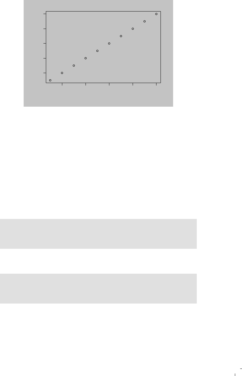
100 Dynamic Documents with R and knitr
246810
2
4
6
8
10
Index
1:10
FIGURE 10.1: A plot with the default margin, i.e., par(mar = c(5.1,
4.1, 4.1, 2.1)).
This hook is used to set the margin parameter with par() for R base
graphics (because the default margin is often too big).
10.1.2 Trigger Chunk Hooks
After we have defined a hook, we need to set a chunk option with the
same name to a non-NULL value in order to execute the hook function.
By default all undefined chunk options are NULL, so the chunk below is
equivalent to a chunk with the option margin = NULL, which will not
call the hook we just defined when the chunk is compiled (Figure 10.1):
<<mar-normal>>=
par(bg = "gray")
plot(1:10)
@
However, when we set margin = TRUE, the hook will be called be-
fore the chunk is evaluated because TRUE is not NULL (Figure 10.2):
<<mar-small, margin=TRUE>>=
par(bg = "gray")
plot(1:10)
@
We set the plot background to be gray just to show the margins more
clearly.

Hooks 101
246810
2468
10
Index
1:10
FIGURE 10.2: A plot with a smaller margin using the margin hook
(par(mar = c(4, 4, .1, .1))).
10.1.3 Hook Arguments
Now we explain the four arguments of a chunk hook. Note all four
arguments are optional.
before a logical value: TRUE if the hook is called before a chunk, and
FALSE when a hook is called after a chunk
options a list of current chunk options, e.g., options$label is the cur-
rent chunk label
envir the environment in which the current code chunk is evaluated,
e.g., envir$x is the object x in the current chunk (if it exists)
name the name of the current hook function
A chunk is called twice for a chunk: once before a chunk and once after
a chunk. In the above margin hook, par() was called before a chunk is
evaluated, so the plots will use the parameters set by par(). If we set
par() after a chunk, it will be too late (hence useless) because the plots
have already been drawn.
10.1.4 Hooks and Chunk Options
Since chunk hooks are called as long as the corresponding chunk op-
tions are not NULL, we can set these chunk options globally if we want
the chunk hooks to be applied to all chunks in a document, e.g.,

102 Dynamic Documents with R and knitr
opts_chunk$set(margin = TRUE)
Note that non-NULL does not necessarily mean TRUE; in the above
example, we can also set margin = 1 or margin = ’hello’, and so on,
because these values are not NULL either.
Since knitr accepts arbitrary chunk options, the options argument
in chunk hooks can be very flexible. The previous example did not
actually make good use of the chunk option margin, because this option
was basically ignored in the hook. Now we extend the hook a little bit,
with margin being a vector to be passed to par(mar = ...):
knit_hooks$set(margin = function(before, options, envir) {
if (before) {
m <- options$margin
if (is.numeric(m) && length(m) == 4L) {
par(mar = m)
}
} else NULL
})
Instead of using a fixed value c(4, 4, .1, .1) for the margin pa-
rameter, we can use any numeric vectors of length 4 now, e.g.,
<<mar-numeric, margin=c(2, 3, 1, .1)>>=
plot(1:10)
@
Then before this chunk is evaluated, par(mar = c(2, 3, 1, .1))
will be called first.
10.1.5 Write Output
Since a chunk hook is a function, it also has a returned value. If the
value returned is character, it will be written to the output. The previ-
ous hooks did not write anything to the output because they did not
return character values (par() returns a list).
Below is a hook that returns character values: a down brace
z}|{
before a chunk and an up brace
|{z}
after a chunk.
knit_hooks$set(brace = function(before, options, envir) {
if (before) {
"\\noindent\\downbracefill{}\n\n"

Hooks 103
} else {
"\n\n\\noindent\\upbracefill{}\n"
}
})
We apply this brace hook to the following chunk:
z }| {
<<test, brace=TRUE>>=
1 + 1
## [1] 2
rnorm(10)
## [1] -0.1738 1.1675 0.8677 -0.8149 -1.6213 0.8553
## [7] -1.8358 -0.7550 -1.6286 -0.6447
@
| {z }
Chunk hooks that return character values allow us to write anything
we want to the chunk output. One important application is to write im-
ages to the output, which we have created through R code in the chunk.
The character values may be like \includegraphics{...} (L
A
T
E
X), <img
src=’...’ /> (HTML) or  (Markdown), etc. This is the trick
we will use for the next few sections, such as saving rgl and GGobi
plots.
10.2 Examples
In this section we give some examples of chunk hooks, most of which
have been predefined in knitr, i.e., we can use them directly after knitr
has been loaded.
10.2.1 Crop Plots
Some R users may have been suffering from the extra white margins
in R plots, especially in base graphics (ggplot2 is usually better in this
aspect). The default graphical option mar is about c(5, 4, 4, 2) as

104 Dynamic Documents with R and knitr
165 170 175 180 185
-35
-30
-25 -20 -15
-10
long
lat
FIGURE 10.3: The original plot produced in R, with a large white mar-
gin.
we mentioned in Figure 10.1 (also see ?par), which is often too big.
Instead of endlessly tweaking par(mar), we may consider the program
pdfcrop, which can crop the white margin automatically (http://www.
ctan.org/pkg/pdfcrop). In knitr, we can set up the hook hook_pdfcrop()
to work with a chunk option, say, crop.
knit_hooks$set(crop = hook_pdfcrop)
Now, we compare two plots produced by the same code chunk be-
low. The first one is not cropped (Figure 10.3); then the same plot is
produced but with a chunk option crop = TRUE, which will call the
cropping hook (Figure 10.4).
par(mar = c(5, 4, 4, 2)) # large margin
plot(lat ~ long, data = quakes, pch = 20, col = rgb(0, 0,
0, 0.2))
As we can see, the white margins are gone (to better see the differ-
ence, we have put a frame box around each plot). If we use par(), it
might be hard and tedious to figure out a reasonable amount of margin

Hooks 105
165 170 175 180 185
-35 -30 -25 -20 -15 -10
long
lat
FIGURE 10.4: The cropped plot; obviously the white margins on the
top and right have been removed.
such that no label is cropped due to a too-small margin, nor do we get
too large a margin.
10.2.2 rgl Plots
With the hook hook_rgl(), we can easily save snapshots from the rgl
package (Adler and Murdoch, 2014). The rgl hook is a good exam-
ple of taking care of details by carefully using the options argument
in the hook; for example, we cannot directly set the width and height
of rgl plots in rgl.snapshot() or rgl.postscript(), so we make use of the op-
tions fig.width, fig.height, and dpi to calculate the expected size of
the window, then resize the current window by par3d(), save the plot,
and finally return a character string containing the appropriate code
to insert the plot into the output. Here is a quick and dirty version of
hook_rgl():
knit_hooks$set(rgl = function(before, options, envir) {
library(rgl)
if (before || rgl.cur() == 0)
return() # return nothing before a chunk
name <- paste(options$fig.path, options$label, sep = "")

106 Dynamic Documents with R and knitr
FIGURE 10.5: An rgl plot captured by hook_rgl(): this hook function
calls rgl.snapshot() in rgl to save the snapshot into a PNG image.
rgl.snapshot(paste(name, ".png", sep = ""), fmt = "png")
paste("\\includegraphics{", name, "}\n", sep = "")
})
The real hook function in knitr is much more complicated than this
due to a lot of details to be taken into consideration. Below is an exam-
ple of how to save rgl plots using the rgl hook. First we define a hook
named rgl for the function hook_rgl():
knit_hooks$set(rgl = hook_rgl)
Then we only have to set the chunk option rgl = TRUE and the cap-
tured plot is shown in Figure 10.5.
library(rgl)
demo("bivar", package = "rgl", echo = FALSE)
par3d(zoom = 0.7)
10.2.3 Manually Save Plots
We have explained how R plots are recorded in Section 7.2. In some
cases, it is not possible to capture plots by recordPlot() (such as rgl plots),
but we can save them using other functions. To insert these plots into
the output, we need to set up a hook first like this (see the help page
?hook_plot_custom for details):

Hooks 107
FIGURE 10.6: A plot created and exported by GGobi, and written into
L
A
T
E
X by the hook hook_plot_custom().
knit_hooks$set(custom_plot = hook_plot_custom)
Then we set the chunk option custom_plot = TRUE, and manually
write plot files in the chunk. Here we show an example of capturing
GGobi plots using the function ggobi_display_save_picture() in the rggobi
package (Temple Lang et al., 2014):
<<ggobi-plot, custom_plot=TRUE, fig.ext='png'>>=
library(rggobi)
data("flea", package = "tourr")
ggobi(flea)
Sys.sleep(1) # wait for snapshot
ggobi_display_save_picture(path = fig_path(".png"))
@
Figure 10.6 is the plot output from GGobi. Two things to note here
are:
1. we have to make sure the plot filename is from fig_path(),
which is a convenience function to return the figure path for
the current chunk (a combination of the chunk label, fig.path
and fig.ext);

108 Dynamic Documents with R and knitr
2. we need to set the chunk option fig.ext (figure file exten-
sion) because knitr will be unable to figure out its value au-
tomatically (we are not using any graphical devices).
We can even save a series of images to make an animation with the
option fig.show = ’animate’ (Section 7.3.1); below is an example of
zooming into a scatterplot using rgl (for the real animation, see knitr’s
main manual):
## use chhunk options: custom_plot=TRUE, fig.ext='png',
## out.width='2.5in', fig.show='animate', fig.num=20
library(animation) # adapted from demo('rgl_animation')
data(pollen)
uM <- matrix(c(-0.37, -0.51, -0.77, 0, -0.73, 0.67, -0.1,
0, 0.57, 0.53, -0.63, 0, 0, 0, 0, 1), 4, 4)
library(rgl)
open3d(userMatrix = uM, windowRect = c(0, 0, 400, 400))
plot3d(pollen[, 1:3])
zm <- seq(1, 0.05, length = 20)
par3d(zoom = 1) # change the zoom factor gradually later
for (i in 1:length(zm)) {
par3d(zoom = zm[i])
Sys.sleep(0.05)
rgl.snapshot(paste(fig_path(i), "png", sep = "."))
}
10.2.4 Optimize PNG Plots
The free software OptiPNG is a PNG optimizer that re-compresses im-
age files to a smaller size, without losing any information (http://
optipng.sourceforge.net/). In knitr, the hook function hook_optipng()
is a wrapper around OptiPNG to compress PNG plots, and OptiPNG
has to be installed beforehand; for Windows users, the executable has
to be in the PATH variable. We can set up the hook as usual:
knit_hooks$set(optipng = hook_optipng)
Then we can either set the chunk option optipng = TRUE to enable
it for a chunk, or pass a character string to this option so that it is used
by OptiPNG as additional command line arguments. For example, we
can use optipng = ’-o7’ to specify the highest level of optimization.
See the documentation of OptiPNG for all possible arguments.

Hooks 109
FIGURE 10.7: Adding elements to an existing rgl plot: if we do not open
a new device, latter elements will be added to the existing device.
10.2.5 Close an rgl Device
The default rgl hook hook_rgl() does not close the rgl device before draw-
ing a new plot, which may be problematic, because the latter plot is
drawn on the previous scene. For example, we get one plot with two
spheres (Figure 10.7) when we execute the following two lines together,
but two plots with one sphere in each if we close the first plot and run
the second line:
rgl.spheres(0, 0, 0)
rgl.spheres(0, 2, 0)
Normally different code chunks use different graphical devices, so
graphical elements in a latter chunk will not be added to a previous
chunk, but this is not true for rgl plots. In order to close the device
before drawing plots, we have to tweak the hook a little bit, e.g.,
knit_hooks$set(rgl = function(before, options, envir) {
# if a device was opened before this chunk, close it
if (before && rgl.cur() > 0)
rgl.close()
hook_rgl(before, options, envir)
})
The function rgl.cur() returns the current device id; if it is greater
than 0, it means there is an existing device, and we can close it by
rgl.close().

110 Dynamic Documents with R and knitr
10.2.6 WebGL
We introduced how to save static rgl plots in Section 10.2.2. In fact, we
can also export the rgl 3D plot into WebGL (http://en.wikipedia.
org/wiki/WebGL) using the writeWebGL() function, so that the plot can
be reproduced in a Web browser that supports WebGL. For example,
we can rotate and zoom in/out the plot.
The hook function hook_webgl() in knitr is a wrapper to the WebGL
function in rgl. With this hook, we can capture a 3D scene into the
HTML output.

11
Language Engines
We can work with a lot of languages and tools in knitr, including but
not limited to R, although knitr is an R package and has to be run within
the R environment in the first place. Currently knitr supports Python,
Ruby, Haskell, awk/gawk, sed, shell scripts, Perl, SAS, TikZ, Graphviz,
and C++, etc. We have to install the corresponding software package in
advance to use an engine.
11.1 Design
Like chunk hooks, all language engines are essentially R functions in
knitr. These functions pass the code chunk to external programs, run
the code there, get the results back, and write to the output. In most
cases, the code is passed to external programs via the system() function.
For example, we can pass code to bash via the -c option.
system("bash -c 'ls ~ | grep ^D'", intern = TRUE)
## [1] "Desktop" "Downloads" "Dropbox"
For those who are not familiar with bash scripts, the code ls ~ |
grep ^D means to list files under the home directory (~) and pass the
filenames to grep through the pipe (|) to match those starting with the
letter D; ls and grep are standard Linux commands.
The chunk option engine can be used to specify the language engine
for a chunk, e.g., the chunk below uses engine = ’bash’:
ls ∼ | grep ^D
## Desktop
## Downloads
## Dropbox
111

112 Dynamic Documents with R and knitr
Then the code in the chunk will be treated as a bash script instead of
an R script. The output rendering is similar to R output: the source code
is passed to the source hook (i.e., knit_hooks$get(’source’)), and the
output is passed to the output hook (knit_hooks$get(’output’)). The
built-in output hooks are fairly general in terms of document formats;
we do not need to think about whether the output is to be L
A
T
E
X or
HTML or Markdown; everything will be automatically and properly
marked up according to the output document format.
11.1.1 The Engine Function
All language engines are stored in the object knit_engines, which has
the $get() and $set() methods like knit_hooks (chunk hooks) and
opts_chunk (chunk options); e.g., we can get the Python engine by
knit_engines$get(’python’), or override the built-in Python engine
by knit_engines$set(python = function(options) {...}).
An engine has one argument: options, which is a list of current
chunk options. Among all options there is one special option named
code, which is the code (as a character string) of the current chunk and
plays the central role in the language engine.
To continue the bash example, we can define a preliminary engine
like this:
knit_engines$set(bash = function(options) {
code <- paste(options$code, collapse = "\n")
out <- system(paste("bash -c", shQuote(code), sep = " "),
intern = TRUE)
paste(c(code, out), collapse = "\n")
})
What this engine does is to concatenate the command bash -c with
the source code, execute the whole command via system(), and return
both the source code and output as one character string separated by
line breaks. The returned character string will be written into the output
document.
The real bash engine is more complicated than this: it has to take
care of some chunk options such as echo, results, include, cache,
and so on. For example, when echo = FALSE, the source code should
be hidden, and when cache = TRUE, the code chunk should be cached.
In all, the behavior of these language engines is very similar to the R
engine, although the support is not as comprehensive as R.
Note in particular the cache of language engines other than R: in
most cases, only the side effects such as printing are cached, due to the

Language Engines 113
fact that it is difficult for R to know which objects are created in a code
chunk if the code is not written in R. In other words, objects are lost
when we exit from a chunk (unless they are exported to files). Normally
we will not be able to reuse an object created from previous chunks.
The reason that we can use R objects across different chunks is that all
R chunks are evaluated in the same R session, but other languages are
evaluated in separate sessions per chunk basis.
11.1.2 Engine Options
For language engines, there are two common chunk options:
engine.path specifies the full path to the engine program as a character
string; this may be useful to Windows users when the program to be
called is not in the environmental variable PATH (i.e., the program can-
not be run without full path in the command line), or to Linux users
when there are multiple versions of one program installed and we do
not want to use the default version; in both cases, we can set the chunk
option engine.path = ’full/path/to/program’, e.g., engine.path
= ’/usr/bin/ruby1.9.1’ (if there are multiple versions of Ruby) or
engine.path = ’C:/Program Files/SASHome/x86/9.3/sas.exe’ (to
specify the full path of SAS);
engine.opts additional options to be passed to an engine; its value
depends on the specific engine; for most engines, it contains addi-
tional command line arguments, e.g., for engine = ’ruby’, we can
set engine.opts = ’-v’ for Ruby to print its version number, then
turn on the verbose mode.
11.2 Languages and Tools
Most languages and tools are supported through the system() interface,
as mentioned in the last section. There are a few exceptions, however,
such as C++ and TikZ.
11.2.1 C++
C++ is supported in knitr through the Rcpp package (Eddelbuettel
et al., 2015). When we set engine = ’Rcpp’, the function sourceCpp()
in Rcpp is used to compile C++ code chunks, which in fact calls R CMD

114 Dynamic Documents with R and knitr
SHLIB internally to build a shared library and load it into R for future
use.
Below is an example for the Fibonacci series (x
i
= x
i−1
+ x
i−2
, x
0
=
0 and x
1
= 1) in C++ with Rcpp:
#include <Rcpp.h>
// [[Rcpp::export]]
int fibCpp(const int x) {
if (x == 0 || x == 1) return(x);
return (fibCpp(x - 1)) + fibCpp(x - 2);
}
After it is compiled, we can call the function fibCpp() in R directly
because we have marked it with the Rcpp::export attribute.
fibCpp(10L)
## [1] 55
system.time(fibCpp(27L))
## user system elapsed
## 0.001 0.000 0.001
Below is the version implemented in pure R:
fibR <- function(x) {
if (x == 0L || x == 1L)
return(x)
return(fibR(x - 1L) + fibR(x - 2L))
}
Unsurprisingly, the R version is much slower, although the numeric
results are the same:
fibR(10L)
## [1] 55
system.time(fibR(27L))
## user system elapsed
## 0.708 0.000 0.708

Language Engines 115
Finally, we can pass additional arguments to sourceCpp() via the
chunk option engine.opts. For example, we can specify engine.opts
= list(showOutput = TRUE) to show the output of R CMD SHLIB (note
showOutput is an argument of sourceCpp()).
11.2.2 C/Fortran
There are two simple language engines c and fortran for the C lan-
guage and Fortran, respectively. These engines are nothing but wrap-
pers for the command R CMD SHLIB and the R function dyn.load(). What
they do is to write the code chunk to a temporary file, run R CMD SHLIB
to compile it, and use dyn.load() to load the compiled library (a .dll or
.so file). To use these engines, you have to make sure you have the
C/Fortran compilers in your system, such as GCC.
# the compilers in the environment in which this book
# was written
Sys.which("gcc")
## gcc
## "/usr/bin/gcc"
Sys.which("gfortran")
## gfortran
## "/usr/bin/gfortran"
Below are two examples demonstrating the usage of these two en-
gines. First, we set the chunk option engine = ’c’ for this example:
/* calculate the square of a number */
void my_square(double *x) {
*x = *x * *x;
}
After compiling the above code chunk, we can call the C function
my_square() via the .C() interface:
.C("my_square", 9)
## [[1]]
## [1] 81
.C("my_square", 123)

116 Dynamic Documents with R and knitr
## [[1]]
## [1] 15129
Next, we show a Fortran example by setting the chunk option engine
= ’fortran’ for the chunk below:
C Fortran test
subroutine fexp(n, x)
double precision x
C output
integer n, i
C input value
do 10 i = 1, n
x = dexp(dcos(dsin(dble(float(i)))))
10 continue
return
end
And we can call the Fortran sub-routine via the .Fortran() interface:
res <- .Fortran("fexp", n = 100000L, x = 0)
str(res)
## List of 2
## $ n: int 100000
## $ x: num 2.72
11.2.3 Interpreted Languages
C++, C, and Fortran belong to compiled languages, and there are other
languages that are interpreted languages. For these languages, we can
execute the code without compiling it. Examples include awk and shell
scripts. There are also some languages that belong to both categories,
such as Python. Table 11.1 lists some interpreted languages supported
by knitr via the system() interface.
For example, a Perl chunk is executed with perl -e code where
code is the character string of the code chunk. For awk and sed, the
argument after the program is treated as the source code, so they do
not need an argument name for the code, e.g., awk ’END{print NR;}’
README counts the number of lines in the file README. For SAS, the
code chunk is written into a file tempfile.sas, and executed as sas -SYSIN
tempfile.sas. There are three shell variants: sh, bash, and zsh.

Language Engines 117
TABLE 11.1: Interpreted languages supported by knitr: the language
name, engine name, and the command line argument to execute code.
Language Engine Code argument
Python python -c
Ruby ruby -e
(g)awk (g)awk
sed sed
shell sh/bash/zsh -c
Perl perl -e
Haskell haskell -e
CoffeeScript coffee -e
Groovy groovy -e
Node.js node -e
Scala scala -e
SAS sas -SYSIN
As we mentioned before, the engine name itself may not be the ex-
ecutable, so we may need to specify the path to the real path of the
program. For Haskell, haskell is not the program to run Haskell,
whereas ghc is, so we need to specify both engine = ’haskell’ and
engine.path = ’ghc’.
We give a few examples of the above languages. Here is a Python
chunk (chunk option engine = ’python’):
x = ’hello, python world!’
print x
print x.split(’ ’)
## hello, python world!
## ['hello,', 'python', 'world!']
Here is a Ruby chunk:
x = ’hello, ruby world!’
p x.split(’ ’)
## ["hello,", "ruby", "world!"]
Below is an awk script to count the number of non-empty lines in
the NEWS.Rd file of the knitr package: in awk, NF denotes the number
of fields on a line; when it is not 0, the variable i increases by 1, and
that is why the script counts the non-empty lines in the file. Note that

118 Dynamic Documents with R and knitr
we used engine.opts = shQuote(system.file(’NEWS.Rd’, package
= ’knitr’)) for this chunk; i.e., we get the path to the NEWS.Rd file
from R, quote it by shQuote(), and pass it to awk as the second argument
(remember the first argument is the code chunk), which means the file
to be read into awk.
# how many non-empty lines in the NEWS file?
NF {
i = i + 1
}
END { print i }
## 8
Finally we have a Perl code chunk:
$test = "jello world";
$test =∼ s/j/h/;
print $test
## hello world
11.2.4 Stan
We can use the rstan package (Guo et al., 2014) to compile models of
Stan, a relatively new programming language featuring Bayesian sta-
tistical inference. There is a language engine called stan in knitr that
allows us to write Stan models in code chunks. We can certainly com-
pile a Stan model in a normal R code chunk without using a special
language engine, by saving the model as a file, or writing the model as
a long character string in R code. Both ways have their disadvantages:
it is not convenient for the reader to see the real model in the report
if it is in an external file, and it is cumbersome to write a model as a
long character string of multiple lines in R. The stan engine makes it
possible to write the model as a code chunk, which solves both prob-
lems mentioned before. Here is a simple example of sampling from the
posterior distribution of the parameter p (probability of X = 1) of a
Bernoulli distribution:
<<engine='stan', engine.opts = list(x = 'ex1')>>=
data {
int<lower=0,upper=1> X[20];

Language Engines 119
}
parameters {
real<lower=0,upper=1> p;
}
model {
X ∼ bernoulli(p);
}
@
Besides the chunk option engine = ’stan’, we also specified the
option engine.opts = list(x = ’ex1’). Here x means the name of
the Stan model to be saved in the R session. This code chunk will pass
the model to the function stan_model() in rstan, and save the model to
the object ex1. That is why we can use the object ex1 in the next chunk:
library(rstan)
fit <- sampling(ex1, data = list(X = rbinom(20, 1, 0.3)))
SAMPLING FOR MODEL 'anon_model' NOW (CHAIN 1).
Iteration: 1 / 2000 [ 0%] (Warmup)
Iteration: 200 / 2000 [ 10%] (Warmup)
Iteration: 400 / 2000 [ 20%] (Warmup)
Iteration: 600 / 2000 [ 30%] (Warmup)
Iteration: 800 / 2000 [ 40%] (Warmup)
Iteration: 1000 / 2000 [ 50%] (Warmup)
Iteration: 1001 / 2000 [ 50%] (Sampling)
....
print(fit)
Inference for Stan model: anon_model.
4 chains, each with iter=2000; warmup=1000; thin=1;
post-warmup draws per chain=1000,
total post-warmup draws=4000.
mean se_mean sd 2.5% 25% 50% 75%
p 0.36 0.00 0.10 0.18 0.29 0.36 0.43
lp__ -14.93 0.02 0.73 -16.99 -15.12 -14.65 -14.47
97.5% n_eff Rhat
p 0.57 1498 1
lp__ -14.42 1703 1
....

120 Dynamic Documents with R and knitr
We generated 20 random data points from the Bernoulli distribution
with p = 0.3, and used them as the sample data Y for the Bayesian in-
ference. You can see from the sampling output that the posterior mean
of p is near 0.3.
11.2.5 TikZ
We introduced the tikzDevice package in Section 7.6, which enables us
to convert R graphics to TikZ (Tantau, 2008). In fact, we can write raw
TikZ code directly in knitr with the engine tikz.
What the tikz engine does internally is: use a L
A
T
E
X template to in-
sert the code chunk and compile the tex document to PDF. By default it
uses the template in knitr (named tikz2pdf.tex under the misc directory
in knitr’s installation directory):
f <- system.file("misc", "tikz2pdf.tex", package = "knitr")
cat(readLines(f), sep = "\n")
\documentclass{article}
\include{preview}
\usepackage[pdftex,active,tightpage]{preview}
\usepackage{amsmath}
\usepackage{tikz}
\usetikzlibrary{matrix}
\begin{document}
\begin{preview}
%% TIKZ_CODE %%
\end{preview}
\end{document}
The line %% TIKZ_CODE %% will be replaced by the TikZ code chunk.
If the default template is not satisfactory, we can provide a template via
the chunk option engine.opts, e.g., engine.opts = list(template =
’path/to/tikz/template.tex’). Then this T
E
X file is compiled to PDF
via the R function tools::texi2pdf(). If the specified figure file exten-
sion (chunk option fig.ext) is not pdf, ImageMagick (via its convert
utility) will be called to convert the PDF file to other file formats such
as PNG, e.g., when the document format is HTML.
Figure 11.1 is a diagram drawn from raw TikZ code below:
\usetikzlibrary{arrows}
\begin{tikzpicture}[node distance=2cm, auto,>=latex’, thick]
\node (P) {$P$};

Language Engines 121
PB
AC
ˆ
P
f
g
f
g
ˆg
ˆ
f
k
FIGURE 11.1: A diagram drawn with TikZ: the source code is written
into a *.tex file and compiled to PDF by L
A
T
E
X.
\node (B) [right of=P] {$B$};
\node (A) [below of=P] {$A$};
\node (C) [below of=B] {$C$};
\node (P1) [node distance=1.4cm, left of=P, above of=P]
{$\hat{P}$};
\draw[->] (P) to node {$f$} (B);
\draw[->] (P) to node [swap] {$g$} (A);
\draw[->] (A) to node [swap] {$f$} (C);
\draw[->] (B) to node {$g$} (C);
\draw[->, bend right] (P1) to node [swap] {$\hat{g}$} (A);
\draw[->, bend left] (P1) to node {$\hat{f}$} (B);
\draw[->, dashed] (P1) to node {$k$} (P);
\end{tikzpicture}
To develop tikz graphics, the programs qtikz or ktikz can be help-
ful, since they provide a graphical user interface (an editor), which al-
lows one to preview the results.
11.2.6 Graphviz
Graphviz (Ellson et al., 2002) is an open source and popular graph visu-
alization software package (http://www.graphviz.org); it is powerful
for drawing diagrams of abstract graphs and networks. Graphviz con-
tains a few “filters,” such as dot, to draw directed graphs, and neato
to draw undirected graphs. When engine = ’dot’, dot is used by de-
fault; to use other filters, we can set, e.g., engine.path = ’neato’.
Figure 11.2 is an example taken from the documentation of Graphviz.

122 Dynamic Documents with R and knitr
a
b x y
z
hi
hello
world
multi-line
label
FIGURE 11.2: A diagram drawn with dot in Graphviz (taken from the
dot manual).
We used fig.ext = ’pdf’ here to produce a PDF graph file, and we
can change it to other file formats like PNG as well.
digraph test123 {
a -> b -> c;
a -> {x y};
b [shape=box];
c [label="hello\nworld",color=blue,fontsize=24,
fontname="Palatino-Italic",fontcolor=red,style=filled];
a -> z [label="hi", weight=100];
x -> z [label="multi-line\nlabel"];
edge [style=dashed,color=red];
b -> x;
{rank=same; b x}
}
If you want to draw diagrams in HTML documents generated from
R Markdown, you may consider the DiagrammeR package (https:
//github.com/rich-iannone/DiagrammeR), which is an HTML wid-
get package that wraps a few JavaScript libraries (see Section 14.5.3 for
more information about HTML widgets).
11.2.7 Highlight
Highlight is a free and open source software package by Andre Simon
(http://www.andre-simon.de) to do syntax highlighting for a large va-

Language Engines 123
riety of languages, including C, PHP, and R, etc. It can write the output
in either L
A
T
E
X or HTML.
When the chunk option engine = ’highlight’, the highlight pro-
gram is called to generate the highlighted code chunk. The chunk op-
tion engine.opts is a character string to pass additional arguments to
Highlight, e.g., we can specify the input syntax via -S, and the type of
output via -O.
The chunk below was taken from the previous awk example; it uses
the chunk option engine.opts = ’-S awk -O latex’ to tell Highlight
that the input syntax is awk, and the output type is L
A
T
E
X, so that High-
light can produce appropriate L
A
T
E
X commands on keywords. It may be
difficult to see the colors in the printed version of this book, but at least
we can see the first line is italic (comments).
# how many non-empty lines in the NEWS file?
NF {
i = i + 1
}
END { print i }
Note that Highlight generates commands like \hlnum{} (for num-
bers) and \hlstr{} (for strings) to mark up different tokens in the code.
These commands are mostly consistent with knitr’s syntax highlight-
ing commands, but there are a few exceptions, e.g., \hlslc{} (for com-
ments) produced by Highlight is not a part of knitr’s commands, so
we need to define it in the L
A
T
E
X preamble. Similarly, if the Highlight
output is HTML, we need to define CSS styles for the class hl slc.
11.2.8 Other Engines
There are two more engines that are essentially for any language: cat
and asis. The cat engine calls the function cat() to write the code
chunk to a file, and the filename can be provided in the chunk option
engine.opts = list(file = ?). The asis engine does nothing but
just write the code chunk as-is in the output. However, it respects the
chunk options eval and echo: if either of these options is FALSE, the
code chunk will be hidden from the output, which can be useful when
you want to dynamically control whether to show some content in the
output.
For example, we can write the code chunk below to a file named
styles.css through the cat engine:

124 Dynamic Documents with R and knitr
<<engine='cat', engine.opts = list(file = 'styles.css')>>=
p {
margin: 5px 2px 5px 2px;
}
@
The following code chunk will be included in the final output if the
variable internal.only is TRUE (imagine you have a portion of the re-
port content that you only want to show internally in your group):
<<engine='asis', echo = internal.only>>=
Here are some top secrets about our analysis that are hidden
in the public version of this report by setting
'internal.only' to TRUE.
Secret number one: ...
@
11.3 Persistent Sessions
In fact, there is a major flaw in the engines for interpreted languages
introduced before: a new engine session is established for every single
code chunk of this engine. This means all code chunks are independent
in memory, and the variables created in previous chunks will not be
available in latter chunks. The only exception is R code chunks: all of
them are evaluated in the same R session. To address this issue, we
need to open a persistent session for an engine, and keep on running
code chunks in this session. For example, we can create a variable in a
Python code chunk, and continue using it in the next Python chunk.
The runr package (Xie, 2013) is an attempt to solve this problem.
Currently it has experimental support for Bash and Julia code, based
on socket connections. The basic idea is like this (take the Julia engine
as example):
1. Open a background Julia process that starts a socket server
and keeps listening (the background process is detached from

Language Engines 125
the current R session by system(’julia script.jl’, wait
= FALSE));
2. R connects to the Julia socket server via socketConnection(open
= ’w’), and writes the Julia code chunk to the server;
3. Julia receives the code, evaluates it, and writes the standard
output (as plain text) to the socket;
4. R reads from the socket via socketConnection(open = ’r’),
and writes the Julia output to the report just like R code chunk
output;
5. Repeat steps 2–4 if the next Julia code chunk comes in, and
Julia will quit if we send the code quit() to it.
In this way, the Julia session will be live until we explicitly shut it down
from R, and all Julia code chunks will be evaluated in the same Julia
session. The runr package is still at its early stage, and community
contribution is welcome.


12
Tricks and Solutions
In this chapter we show some tricks that can be useful for writing and
compiling reports more easily and quickly, and also solutions to fre-
quently asked questions.
12.1 Chunk Options
There are a number of built-in chunk options in knitr, and we usually
assign values to them in chunk headers, but it is still possible to cus-
tomize these fixed options, e.g., rename the options.
12.1.1 Option Aliases
We may feel some options are very frequently used but the names are
too long to type. In this case we can set up aliases for chunk options
using the function set_alias() in the beginning of a document, e.g.,
set_alias(w = "fig.width", h = "fig.height")
Then we will be able use w and h for the figure width and height,
respectively, e.g.,
<<fig-size, w=5, h=3>>=
plot(1:10)
@
The chunk above is equivalent to:
<<fig-size, fig.width=5, fig.height=3>>=
plot(1:10)
@
127

128 Dynamic Documents with R and knitr
12.1.2 Option Templates
Besides option names, we can also bundle frequently used option val-
ues together as option templates. The object opts_template in knitr
can be used to build such templates. A template is a named collection
of option sets. For example, if there are a large number of plots for
which we want to set the graphical device size to be 7 ×5 inches, and
for other plots, we want the size to be 3.5 ×3 inches. We can certainly
type fig.width = 7, fig.height = 5 for the first group of plots, and
fig.width = 3.5, fig.height = 3 for the second group, but this is
apparently tedious (even with option aliases). In this case we can just
put the two sets of options in templates:
opts_template$set(
fig.large = list(fig.width = 7, fig.height = 5),
fig.small = list(fig.width = 3.5, fig.height = 3)
)
After the templates have been set up, we can simply use the chunk
option opts.label in future chunk headers to reference to them. For
instance, we want the options for large plots in the chunk below:
<<fig-ex, opts.label='fig.large'>>=
plot(1:10)
@
This is equivalent to:
<<fig-ex, fig.width=7, fig.height=7>>=
plot(1:10)
@
12.1.3 Program Chunk Options
Since chunk options can take arbitrary R expressions, we can program
chunk options besides setting fixed values like numbers or logical val-
ues. We show below an example of drawing a table with the gridExtra
package. First we use the tableGrob() function to create a table Grob
(graphical object):
library(gridExtra)
g <- tableGrob(head(iris))

Tricks and Solutions 129
1
2
3
4
5
6
Sepal.Length
5.1
4.9
4.7
4.6
5.0
5.4
Sepal.Width
3.5
3.0
3.2
3.1
3.6
3.9
Petal.Length
1.4
1.4
1.3
1.5
1.4
1.7
Petal.Width
0.2
0.2
0.2
0.2
0.2
0.4
Species
setosa
setosa
setosa
setosa
setosa
setosa
FIGURE 12.1: A table created by the gridExtra package: we create a
table Grob and draw it in a proper graphical device.
Next, we use grid.draw() in the grid package to draw the object to
a plot. Prior to that, we need to determine an appropriate size for the
graphical device; otherwise we might get extra white margins in the
plot. In fact, the convertWidth() and convertHeight() functions in the grid
package can convert the pre-calculated width and height of the Grob
to inches. Therefore, we pass two function calls to the chunk options
fig.width and fig.height instead of using fixed numbers as we usu-
ally do. Figure 12.1 is a table of the first four lines of the iris data
drawn by grid.draw().
<<table, fig.width=convertWidth(grobWidth(g), 'in', TRUE)>>=
## width and height in inches
convertWidth(grobWidth(g), "in", value = TRUE)
## [1] 5.55
convertHeight(grobHeight(g), "in", value = TRUE)
## [1] 1.94
grid.draw(g)
@
The programmable chunk options enable us to program our reports
in many aspects. As one potential application, we may build a lin-
ear regression report including common diagnostic procedures, with
each procedure in a child document (Section 9.3). Then we can decide
whether to include certain procedures based on certain conditions, e.g.,
if we have detected outliers in the regression model, we include an out-
lier module to deal with outliers. The chunk below shows a sketch of
this idea:

130 Dynamic Documents with R and knitr
<<cooks-distance>>=
cookd <- cooks.distance(fit)
# include an outlier procedure if any distance is
# greater than 1
<<outlier, child=if (any(cookd > 1)) 'outlier.Rnw'>>=
@
12.1.4 Code in Appendix
Sometimes we do not want to show the code chunks in the body of
the report, but we do not want to completely hide the code, either. In
this case we can move all code chunks to the appendix, and the chunk
option ref.label can be useful here (Section 9.1.2).
If there are only a small number of code chunks in the document,
we can manually type their labels, e.g.,
<<A, echo=FALSE>>=
1+1
<<B, echo=FALSE>>=
2+2
<<C, echo=FALSE>>=
rnorm(10)
<<show-code, ref.label=c('A', 'B', 'C'), eval=FALSE>>=
@
Here we hide the code in the previous chunks by echo = FALSE,
and gather them into the last chunk by ref.label. Note the last chunk
used the chunk option eval = FALSE so that the code is not evaluated
again.
If there are a lot of code chunks in a document, we can use the func-
tion all_labels() in knitr to obtain all chunk labels in a document, and
pass them to ref.label, e.g.,
<<show-code, ref.label=all_labels()>>=
@
We can set echo = FALSE globally by opts_chunk$set(), and use
echo = TRUE for the last chunk to show the code there. Of course we
can also select chunk labels to include there, e.g., remove the first chunk
by all_labels()[-1].

Tricks and Solutions 131
12.1.5 Local R Options
The chunk option R.options can take a list of R options to be passed
to options() for a code chunk. These options will be applied to the code
chunk, and restored after the chunk, so it can be useful if you want to
temporarily change R options for a particular code chunk.
For example, we use local options width = 30 (the approximate
width for printing) and digits = 2 (the number of digits for printing)
for the following code chunk:
<<R.options = list(width=30, digits=2)>>=
seq(0, 10, length = 20)
## [1] 0.00 0.53 1.05 1.58
## [5] 2.11 2.63 3.16 3.68
## [9] 4.21 4.74 5.26 5.79
## [13] 6.32 6.84 7.37 7.89
## [17] 8.42 8.95 9.47 10.00
@
12.1.6 Dynamic Code
Usually we just type the code in a chunk, or include code from other
chunks by references (Chapter 9). There is yet another way to assign
code to a chunk, using the chunk option named code. This makes it
possible to construct a code chunk dynamically. For example, you can
read the code from an external script:
<<code = readLines('foo.R')>>=
@
12.2 Package Options
Although we did not specifically mention it before, there is an object
named opts_knit in knitr that controls some package-level options,
and its usage is the same as chunk options (opts_chunk).
By default we see a progress bar when we call knitr, and we can sup-
press it by setting opts_knit$set(progress = FALSE). The progress

132 Dynamic Documents with R and knitr
bar shows the progress of knit() so we know which chunk is currently
being compiled if it takes a relatively long time. To see more informa-
tion about chunks such as the source code, we can turn on the verbose
mode by opts_knit$set(verbose = TRUE).
The package option root.dir can be used to set the root working
directory when evaluating code chunks. The default working directory
is the directory of the input document, but we can change it with this
option, e.g., after we set
opts_knit$set(root.dir = "/home/foo/bar/")
Then we can read a data file under that directory without using the
full path, but in general, we recommend putting datasets and source
documents in the same directory, and use this directory as the working
directory.
For the chunks that are not labeled, automatic labels of the form
unnamed-chunk-i will be used. This can be customized via the package
option unnamed.chunk.label, e.g.,
opts_knit$set(unnamed.chunk.label = "fig")
Then the automatic chunk labels will be fig-1, fig-2, and so on.
12.3 Typesetting
In this section we show some solutions to tweaking the typesetting of a
report.
12.3.1 Output Width
A common problem of using knitr in L
A
T
E
X is that the output width may
exceed the page margin. There are three types of widths: the width of
the source code, the text output, and the graphics output. In Section 7.4
we mentioned \maxwidth, which guarantees the graphics output will
not be wider than the page width.
For the width of source code and text output, it is controlled by the
global option width in options() (Section 6.2.2). The default value for
this option is 75, which may be too large for L
A
T
E
X documents unless we
have reset the page margins (e.g., using the geometry package).
When we see the source code or the text output is too wide, we can
use a smaller width option, e.g.,

Tricks and Solutions 133
options(width = 55)
However, this may not work all the time: for the source code, R may
not be able to find an appropriate place to break the source lines; for text
output, the original lines may not contain line breaks (because they are
in the verbatim environments, L
A
T
E
X will not break the lines automat-
ically). For the example below, the text lines will not be wrapped no
matter how small the width option is:
# unable to wrap the source code
x <- "thisistoolongandRisunabletofindaplacetoinsertthelinebreak"
# unable to wrap the output line
cat(x, "---")
## thisistoolongandRisunabletofindaplacetoinsertthelinebreak ---
This is an extreme example. Normally our source code can be for-
matted into several lines. If we have a character string that is too long
in the source code, we can consider breaking it into smaller pieces man-
ually and pasting them together with paste(), e.g.,
x <- paste("this", "is", "too", "long", "and", "R", "is",
"unable", "to", "find", "a", "place", "to", "insert",
"the", "line", "break", sep = "")
An alternative approach is to use the listings style (recall Figure 5.2
and the function render_listings()). We can set the breaklines option to
true for the listings package in the L
A
T
E
X preamble:
\lstset{breaklines=true}
See Figure 12.2 for an example of this option in L
A
T
E
X.
12.3.2 Message Colors
For L
A
T
E
X output, there are three colors defined, corresponding to mes-
sages, warnings, and errors, respectively:
\definecolor{messagecolor}{rgb}{0, 0, 0}
\definecolor{warningcolor}{rgb}{1, 0, 1}
\definecolor{errorcolor}{rgb}{1, 0, 0}
By default messages are black, warnings are magenta, and errors are
red. We can redefine them using the command \definecolor{} in the
L
A
T
E
X preamble.

134 Dynamic Documents with R and knitr
We can set the breaklines option to true to wrap long lines.
p r i n t ( ” asdlfjk sadflkj k l jsd k l w j r kl w j r e k l w jer k l j w r e klj w e r
l k j r w e e l k w j r e l k w j e r e l k w j e r l kwj r e lka sdfa afsd afdafs d
af d d a d f adfsadf afda sdf ” )
[1] " asdlfjk sad flkj kljs d klwjr klwjre klwjer kljwre kljwer
lkjrwee lkwjre lkwjere lkwjer lkwjre lkasdfa afsd afdafs d
afddadf adfsadf afdasdf "
By comparison, this shows breaklines=false:
p r i n t ( ” asdlfjk sadflkj k l jsd k l w j r kl w j r e k l w jer k l j w r e klj w e r l k j r w e e l k wjr e lk w j e r e l k w j e r lk w j r e lkas dfa afsd afd afsd afd d a d f adfsadf afda sdf ” )
[1] " asdlfjk sad flkj kljs d klwjr klwjre klwjer kljwre kljwer
lkjrwee lkwjre lkwjere lkwjer lkwjre lkasdfa afsd afdafs d
afddadf adfsadf afdasdf "
FIGURE 12.2: Break long lines with listings: we can use the function
render_listings() in R and \lstset{breaklines=true} in L
A
T
E
X.
12.3.3 Box Padding
As we introduced in Section 6.2.3, the default L
A
T
E
X style of knitr is
based on the framed package, and that is why we see shaded boxes
underneath all code chunks. If we feel the default padding of the box is
too tight, we can reset the length of \fboxsep{} by \setlength, e.g.,
\setlength\fboxsep{5mm}
## an intentional comment to to to to to to to to to to to to
## reach the page margin
rpois(40, 5)
## [1] 6 4 6 4 9 5 2 4 2 4 4 10 6 3 1 8 8
## [18] 2 7 4 10 6 5 2 7 4 6 4 2 5 8 7 2 3
## [35] 2 7 7 3 3 3
Now we see the gray box is larger, with a padding space of 5 mm.
For HTML output, it is much easier to design the style, e.g., we can
define the class chunk in CSS as this to make the padding 5 mm:
div.chunk {
padding: 5mm;
}

Tricks and Solutions 135
\documentclass{beamer}
\begin{document}
\title{Using knitr in Beamer}
\author{Yihui Xie}
\maketitle
\begin{frame}
\frametitle{Introduction}
This is a normal slide.
\end{frame}
% need the option [fragile] for code output!
\begin{frame}[fragile]
\frametitle{Code chunks}
<<test, out.width='.6\\linewidth', fig.align='center'>>=
par(mar = c(4, 4, .1, .1))
x = rnorm(100)
hist(x, main='', col='lightblue', border='white')
rug(x)
@
\end{frame}
\end{document}
FIGURE 12.3: A simple example of using knitr in beamer slides: note
that we need the option [fragile] after \begin{frame}.
12.3.4 Beamer
Beamer (Tantau et al., 2012) is a popular document class to create slides
with L
A
T
E
X. Using knitr in beamer slides is not very different from other
L
A
T
E
X documents; the only thing to keep in mind is that we need to
specify the fragile option on beamer frames when we have verbatim
output. See Figure 12.3 for the Rnw source of a simple beamer example,
with one page of the output in Figure 12.4.
Due to the limited space in beamer slides, it may be desirable to use
smaller font sizes for the code. In this case we can set a global chunk
option size, e.g.,

136 Dynamic Documents with R and knitr
Code chunks
par(mar = c(4, 4, 0.1, 0.1))
x = rnorm(100)
hist(x, main = "", col = "lightblue", border = "white")
rug(x)
Frequency
−2 −1 0 1 2
0
2015105
FIGURE 12.4: A sample page of beamer slides: a code chunk with a
plot.
<<setup, include=FALSE>>=
opts_chunk$set(size = "footnotesize")
@
Next we show an example of programming the content of output,
which makes it possible to use the beamer command \only{} to show
plots one by one in the same place on the screen (for more information,
see the beamer manual). The basic idea is to replace the graphics com-
mand \includegraphics{} by \only<n>{\includegraphics{}}, with
n being the n-th plot in the current chunk. Below is a modified plot
hook that does this job:
<<setup, include=FALSE>>=
hook_plot <- knit_hooks$get("plot") # the default hook
# tweak and reset the default hook
knit_hooks$set(plot = function(x, options) {
txt <- hook_plot(x, options)
if (options$fig.cur <= 0)
return(txt)

Tricks and Solutions 137
#' add \only<n> before \includegraphics
gsub("(\\\\includegraphics[^}]+})",
sprintf("\\\\only<%d>{\\1}", options$fig.cur),
txt)
})
@
One key here is the option fig.cur, which is an internal chunk op-
tion (not specified by users) providing the current figure number. The
substitution of \includegraphics{} was done through regular expres-
sions. After we have modified the plot hook, the plot commands in
L
A
T
E
X output will be changed accordingly.
12.3.5 Suppress Long Output
For those who have read the book “Modern Applied Statistics with S”
(MASS) by Venables and Ripley (2002), you may have noticed that the
authors omitted parts of the output in the book in several places, be-
cause the output will otherwise be too long. For example, the data
frame painters on page 17 has 54 rows, but only the first 5 rows were
shown on that page, and the rest of the rows were omitted (the omis-
sion was denoted by ....). We can automate this job by redefining the
output hook in knitr (Section 5.3), e.g.,
# the default output hook
hook_output <- knit_hooks$get("output")
knit_hooks$set(output = function(x, options) {
# print the first 5 lines by default
if (is.null(n <- options$out.lines))
n <- 5
x <- unlist(stringr::str_split(x, "\n"))
if (length(x) > n) {
# truncate the output
x <- c(head(x, n), "....\n")
}
# paste first n lines together
x <- paste(x, collapse = "\n")
hook_output(x, options)
})
Then we can achieve a similar effect of the example in the MASS
book:

138 Dynamic Documents with R and knitr
library(MASS)
painters
## Composition Drawing Colour Expression
## Da Udine 10 8 16 3
## Da Vinci 15 16 4 14
## Del Piombo 8 13 16 7
## Del Sarto 12 16 9 8
....
The basic idea of the hook defined above is, if the number of lines of
the output is greater than 5, we extract the first 5 lines by head(x, 5),
and append .... to the output vector, then pass the modified output
to the default output hook function hook_output(), which was obtained
before we reset the output hook. We do not have to hard-code the num-
ber of lines to be 5, so we also check if the chunk option out.lines is
NULL; if it is not, it is supposed to be a number to specify the number
of lines to keep in the output. For example, we print the first 10 lines
instead:
<<print-painters, out.lines=8>>=
library(MASS)
painters
@
Note this hook applies to all document formats (Rnw and Rmd,
etc.), because we do not have any document-specific code in the new
definition; for different document formats, knit_hooks$get(’output’)
will be different as well, hence the new hook is portable.
12.3.6 Escape Special Characters
As introduced in Section 5.3, the inline hook function is used to write
inline results into the output. By default, it writes characters as is, and
sometimes we may want to escape special characters in L
A
T
E
X or HTML,
e.g., an inline R code fragment produces a percentage 30%, and we have
to write % as \% in L
A
T
E
X, otherwise it means L
A
T
E
X comments.
It is unclear whether we should escape special characters or not, e.g.,
we may generate a L
A
T
E
X equation from inline R code, in which case we
must not escape special characters such as backslashes. Anyway, if we
do want to escape them, we can create a new inline hook function,
e.g.,

Tricks and Solutions 139
# get the default inline hook
hook_inline <- knit_hooks$get("inline")
# build a new inline hook
knit_hooks$set(inline = function(x) {
if (is.character(x))
x <- knitr:::escape_latex(x)
hook_inline(x)
})
An internal function escape_latex() was used to escape special L
A
T
E
X
characters, and the escaped text strings will be passed to the default
inline hook. We only added one step before the default hook function,
and all features of the default hook will be preserved, such as automatic
scientific notation (Section 6.1).
Similarly, if we are writing an R HTML document instead, we can
call the escape_html() function.
12.3.7 The Example Environment
When writting textbooks or tutorials, it can be useful if we number
the R code chunks like theorems and equations. It is easy to define an
“Example” environment in the L
A
T
E
X preamble, e.g., using the amsthm
package:
\usepackage{amsthm}
\newtheorem{rexample}{R Example}[section]
Then we can use this new environment rexample in our document:
\begin{rexample}
<<test, eval=TRUE>>=
1 + 1
rnorm(10)
@
\end{rexample}
In fact, we can automate this job with a chunk hook function, so that
we do not have to type the environment again and again. The rexample
hook below writes the environment automatically for a chunk with a
non-NULL chunk option rexample:
knit_hooks$set(rexample = function(before, options, envir) {
if (before) {

140 Dynamic Documents with R and knitr
sprintf("\\begin{rexample}\\label{%s}\\hfill{}",
options$label)
} else "\\end{rexample}"
})
Basically this hook writes \begin{rexample} before a chunk, and
\end{rexample} after it. Additionally, it writes a label for the environ-
ment so that we can reference it later, and the label is the chunk label.
Now we can apply it to a chunk, e.g.,
<<test, rexample=TRUE>>=
1 + 1
@
Figure 12.5 shows a sample page that used this hook function. We
can see the R code chunks are numbered after the section numbers,
which is due to the [section] option in the definition of the rexample
environment. Because the rexample environments also come with la-
bels, we can use \ref{} for cross references.
It is also possible to create a similar hook for R HTML documents,
but since HTML is not primarily for typesetting purposes, it is not easy
to get the automatic numbering as in L
A
T
E
X. Anyway, we can use our
own counter in R, e.g.,
## an example counter for HTML
example_count <- 0
knit_hooks$set(rexample = function(before, options, envir) {
if (before) {
# increment by 1
example_count <<- example_count + 1
sprintf("<div>Example %d</div>", example_count)
} else ""
})
12.3.8 The Docco Style
Besides L
A
T
E
X documents, you can also use typeset HTML documents.
There is a function rocco() in knitr that provids a two-column layout
for HTML documents. This style was borrowed from a literate pro-
gramming package named Docco (https://github.com/jashkenas/
docco). The narratives and code are arranged in separate columns, so
that you can keep on reading either the narratives or the code in one

Tricks and Solutions 141
Using the Example Environment with knitr
Yihui Xie
January 2, 2013
1 Introduction
This is a test of theRExample environment.
1.1 Go!
R Example 1.1.
1 + 1
## [1] 2
Look at Example 1.1!
1.2 Ha!
R Example 1.2.
x = rnorm(10)
Move on!
R Example 1.3.
sd(x) # standard deviation
## [1] 1.124
How about 1.2 and 1.3?
If you want to use this R Example environment for all code chunks, make
rexampleaglobal chunk option in the setup chunk.
1
FIGURE 12.5: R code chunks in the R Example environments: the ex-
amples are numbered following the section numbers.
column. You can hide either column with a keyboard shortcut. Figure
12.6 is a screenshot of a package vignette in knitr that uses this style:
vignette("docco-classic", package = "knitr")
12.4 Utilities
There are a few utility functions in knitr to complete miscellaneous
tasks such as writing BibT
E
X databases for R packages, base64 encoding

142 Dynamic Documents with R and knitr
FIGURE 12.6: The Docco style for HTML output: the narratives are in
the left column, and the R code is in the right column. You can render
such a page from R Markdown using the function rocco() in knitr.

Tricks and Solutions 143
images for HTML output, and compiling source documents to the final
output.
12.4.1 R Package Citation
The function write_bib() is a wrapper to the functions citation() and to-
Bibtex() in base R. By default it collects the packages loaded into the
current R session and extracts their citation information. It also has an
argument named tweak, which determines whether to tweak the de-
fault citation information, e.g., the author name “Duncan Temple Lang”
should be “Duncan {Temple Lang}” in the bibliography database. In-
stead of manually modifying information like this, write_bib() can auto-
matically deal with it.
write_bib(c("filehash", "RGtk2", "rms"))
@Manual{R-filehash,
title = {filehash: Simple key-value database},
author = {Roger D. Peng},
year = {2014},
note = {R package version 2.2-2},
url = {http://CRAN.R-project.org/package=filehash},
}
@Manual{R-RGtk2,
title = {RGtk2: R bindings for Gtk 2.8.0 and above},
author = {Michael Lawrence and Duncan {Temple Lang}},
year = {2014},
note = {R package version 2.20.31},
url = {http://CRAN.R-project.org/package=RGtk2},
}
@Manual{R-rms,
title = {rms: Regression Modeling Strategies},
author = {Frank E. {Harrell, Jr.}},
year = {2015},
note = {R package version 4.3-0},
url = {http://CRAN.R-project.org/package=rms},
}
The second argument of write_bib() is file, and we can pass a file-
name to it to save the bibliography items into a file. By default, it writes
to the standard output.
The advantage of generating the bibliography database using this
function is that we can guarantee we always cite the package versions

144 Dynamic Documents with R and knitr
that we really use in a document. If we hard-code the bibliography, the
citations may be out-of-date after we update R packages.
If we do not want to write the file each time we compile the docu-
ment, we can cache the chunk. Then a natural question is, when should
we, or how can we update the cache? Recall Chapter 8 and one solu-
tion is to put the package version(s) in a chunk option, e.g., if the main
package that we use for a document is called foo, we can write a chunk
like this:
<<write-bib, cache=TRUE, version=packageVersion('foo')>>=
write_bib(c("foo", "other", "packages"), file = "paper.bib")
@
Then whenever the foo package is updated, the cached chunk will
be updated accordingly.
12.4.2 Image URI
It is convenient to publish a PDF report because a PDF document con-
tains everything in one file, including plots in particular, but that is not
true for HTML reports. If an HTML page contains images that are ex-
ternal files, we have to publish these images along with the HTML file,
otherwise the Web browser will not be able to find them. There is a
technology called “Data URI” in Web pages that solves this problem.
In short, we can encode a file into a character (base64) string and in-
clude it in HTML, so that we do not need the original file any more
when publishing the HTML page. In other words, the HTML page is
self-contained just like PDF.
The function image_uri() in knitr was designed to encode images as
base64 strings. Obviously it only applies to HTML output (including
Markdown). We can enable this function in opts_knit:
opts_knit$set(upload.fun = image_uri)
Then if we have plots in HTML output, the image file paths will be
replaced by base64 character strings. Below is an example of encoding
the R logo (a JPEG image):
# encode the R logo
logo <- file.path(R.home("doc"), "html", "logo.jpg")
uri <- image_uri(logo)
# the first 250 characters
uri.sub <- substring(uri, seq(1, 201, 50), seq(50, 250,

Tricks and Solutions 145
50))
cat(uri.sub, sep = "\n")
data:image/jpeg;base64,/9j/4AAQSkZJRgABAQEBKwErAAD
/4QAWRXhpZgAATU0AKgAAAAgAAAAAAAD/2wBDAAUDBAQEAwUEB
AQFBQUGBwwIBwcHBw8LCwkMEQ8SEhEPERETFhwXExQaFRERGCE
YGh0dHx8fExciJCIeJBweHx7/2wBDAQUFBQcGBw4ICA4eFBEUH
h4eHh4eHh4eHh4eHh4eHh4eHh4eHh4eHh4eHh4eHh4eHh4eHh4
12.4.3 Upload Images
Based on the same reason, we designed another function imgur_upload()
to upload images to the website Imgur.com, and this function returns
the URL of the uploaded image. Then, instead of using the image file
path to reference the image (which has the problem mentioned before),
we use a URL that is accessible anywhere as long as we have Internet
connection. To continue the previous example, we can upload the R
logo to Imgur website by:
imgur_upload(logo)
This returns a URL of the form http://i.imgur.com/xxxxx.jpg.
To make things even easier, we can set the package option upload.fun
like we did in the last section:
opts_knit$set(upload.fun = imgur_upload)
Then images will be automatically uploaded to Imgur when we knit
a document. To avoid repeated uploading of the same image, we can
turn on cache.
12.4.4 Compile Documents
For some document formats, there are two steps in compilation. For
example, Rnw documents are compiled through knitr to L
A
T
E
X docu-
ments, which need to be compiled to PDF via L
A
T
E
X. For Rmd docu-
ments, the final product is often HTML instead of Markdown, which is
the direct output of knitr.
To turn the two steps into one, the functions knit2pdf() and knit2html()
can be used. The former will first knit() an Rnw document to a T
E
X
document, and then call texi2pdf() in base R to compile it to PDF; the
latter will knit() an Rmd document to a Markdown document, and call

146 Dynamic Documents with R and knitr
markdownToHTML() in the markdown package to compile Markdown
to HTML.
For users under Unix-like systems, there is a Bash script named knit
under the directory bin of knitr’s installation path; we can find it via:
system.file("bin", "knit", package = "knitr")
## [1] "/home/yihui/R/knitr/bin/knit"
It is an executable script that calls R to load knitr and automatically
uses knit2pdf() or knit2html() based on the filename extension; if we put
this script in the PATH variable, we can call it in command line directly.
For example, I have made a symbolic link under ~/bin/ to this script,
and added this to ~/.bashrc:
PATH=$PATH:$HOME/bin
export PATH
Then we can run knit like other programs in the terminal without
having to start R and type all the commands there.
12.4.5 Construct Code Chunks
So far we have been using files as the input for the knit() function in
knitr. As a matter of fact, there is an alternative argument to receive
the source document, which is named text.
# arguments of knit()
formatR::usage(knit, width = 40)
## knit(input, output = NULL, tangle = FALSE,
## text = NULL, quiet = FALSE, envir = parent.frame(),
## encoding = getOption("encoding"))
If we provide an input file to knit(), it will be read into knitr and
assigned to the text argument eventually. The content of files is usually
fixed, but for the text argument, we can dynamically construct it using
R since it is nothing but a character variable.
Now we show a comprehensive example, which builds a PDF doc-
ument for all the geom examples in the ggplot2 package; see the source
code in Figure 12.7 and a sample page of the output in Figure 12.8. It
may look a little bit complicated at first glance, but the basic idea is
simple:

Tricks and Solutions 147
1. in the setup chunk, we set two global chunk options: tidy =
FALSE (optional) and cache = TRUE (because there are a large
number of example code chunks to run later);
2. in the write-examples chunk, we use apropos() to find all
function names that start with geom_; then we find their help
files and from there extract the examples code with Rd2ex() in
the tools package; finally we construct Rnw chunks using the
function names as section titles and chunk labels, and assign
the source text to a variable ex;
3. in the last step, we knit the source passed from the text argu-
ment and knit() returns the L
A
T
E
X code, which we insert into
the document as a text string by \Sexpr{};
This source document will produce a PDF document of more than 200
pages, taking a few minutes on the first run. Note that it uses the doc-
ument class tufte-handout, which is a L
A
T
E
X class you may have to
install (it is not a standard class that comes by default).
12.4.6 Extract Source Code
We mentioned the function purl() briefly in Section 3.4. Actually it
has an additional argument named documentation, which controls the
level of details of documentation chunks.
args(purl)
## function (..., documentation = 1L)
## NULL
The documentation argument takes three possible values:
0L discard all text chunks, including chunk headers, so the output is
pure program code
1L discard text chunks but preserve chunk headers in the exported
code file
2L keep everything in the source document but put text chunks in rox-
ygen comments (i.e., after #’)
The following chunk shows examples corresponding to three values of
the documentation argument. Note that the chunk headers are written
after ## ----, and text chunks are after #’. When documentation = 2,
the generated R script can be passed to the function spin() to restore the
original document (Section 5.4).

148 Dynamic Documents with R and knitr
\documentclass[a4paper,titlepage]{tufte-handout}
\title{ggplot2 Gallery}
\begin{document}
\maketitle
\tableofcontents
<<setup, include=FALSE>>=
# cache chunks and do not tidy ggplot2 examples code
opts_chunk$set(tidy = FALSE, cache = TRUE)
@
% all geoms in ggplot2
<<write-examples, include=FALSE>>=
library(ggplot2)
ex = lapply(apropos("^geom_"), function(g) {
p = utils:::index.search(g, find.package(), TRUE)
tools::Rd2ex(utils:::.getHelpFile(p), f <- tempfile())
c(sprintf("\\section{%s}\n\n<<%s>>=",
knitr:::escape_latex(g), g),
readLines(f), "@\n\n")
})
@
\Sexpr{knit(text = unlist(ex))}
\end{document}
FIGURE 12.7: The source document of the ggplot2 geom examples: the
Rd2ex() function was used to extract all examples code for the geom
functions, and we construct code chunks using the Rnw syntax for knitr
to compile.

Tricks and Solutions 149
35
30
25
20
mpg
15
10
234
wt
5
4
6
factor(cyl)
8
FIGURE 12.8: A sample page of the ggplot2 documentation: the section
titles, code, and plots are all dynamically generated.

150 Dynamic Documents with R and knitr
src <- c("this is the source document", "<<A, tidy=FALSE>>=",
"1+1", "@", "the end")
cat(purl(text = src, documentation = 0L))
1+1
cat(purl(text = src, documentation = 1L))
## ----A, tidy=FALSE-----------------------------------
1+1
cat(purl(text = src, documentation = 2L))
#' this is the source document
## ----A, tidy=FALSE-----------------------------------
1+1
#' the end
For code chunks that have the chunk option purl = FALSE, their
code will be ignored. For those chunks that have eval = FALSE, their
code will be commented out.
12.4.7 Reproducible Simulation
As we discussed in Chapter 8, it is not trivial to write a report that can
be easily and completely reproducible for others. One challenge is to
make random simulations reproducible. Of course we can use set.seed()
to fix the random seed, but what if we have enabled cache?
The problem is, when should we update a cached chunk that in-
volves random numbers? One sufficient condition is the change of the
random seed, i.e., if the random seed has changed before a chunk, this
chunk should be re-evaluated.
The object rand_seed in knitr was designed for this purpose. This
object is essentially an unevaluated expression:
rand_seed
## {
## if (exists(".Random.seed", envir = globalenv()))
## get(".Random.seed", envir = globalenv())
## }
is.language(rand_seed)

Tricks and Solutions 151
## [1] TRUE
Basically it returns the random seed if it exists. We can assign this
object to a chunk option; because it is an unevaluated expression, each
time a chunk is compiled, this object will be evaluated again (knitr will
always evaluate unevaluated chunk options). Then if the random seed
has changed, knitr will be able to detect the change and update the
cached chunk accordingly. Below is an example:
<<random-cache, cache=TRUE, cache.extra=rand_seed>>=
x <- rnorm(100)
@
Even if we only switched the positions of two cached chunks (with
the code and options untouched), the cache will be invalidated be-
cause the evaluated results of rand_seed will be different for these two
chunks compared to the last run.
12.4.8 R Documentation
R has a standard documentation system, and one thing that can be im-
proved is the examples in the help pages — we can actually run these
examples and put the results in the pages, so that it is easier for the
reader to know the results without having to copy and paste code from
the documentation.
The function knit_rd() was designed for this task: it takes a package
name and extracts all its HTML help pages, then compiles all the ex-
amples. This can be handy for package authors, because it generates
HTML files that can be published on the Web, and they are richer than
the default R documentation. For example, we recompile all the help
pages of the rpart package:
knit_rd("rpart")
We will see a few HTML files under the current working directory.
If there are plots in the examples, they will be base64 encoded and em-
bedded in the pages, so we do not need to take care of additional files
— just upload all these HTML files to a website.
12.4.9 Rst2pdf
Rst2pdf (http://rst2pdf.ralsina.com.ar) is a free software package
to create PDF from reStructuredText. If we write the source document

152 Dynamic Documents with R and knitr
\documentclass{article}
\begin{document}
<<read-demo>>=
library(diagram)
read_demo('flowchart', package = 'diagram',
labels = 'demo-flowchart')
<<demo-flowchart, dev='tikz', cache=TRUE>>=
@
\end{document}
FIGURE 12.9: The flowchart demo in the diagram package: we read
the demo into knitr, assign a label demo-flowchart to it, and insert it
into the document using this label.
in the R reST format (Section 5.2.4), the output from knitr is a *.rst doc-
ument, and we can call Rst2pdf (if installed) to convert it to PDF via the
wrapper function rst2pdf() in knitr, or just call knit2pdf(’foo.Rrst’)
in one step.
12.4.10 Package Demos
Some R packages contain demos, which can be run by the demo() func-
tion, e.g.,
demo("plotmath")
demo("notebook", package = "knitr")
We can insert demos into a source document using the read_demo()
function in knitr, which is simply a wrapper of read_chunk() as intro-
duced in Section 9.2.2.
Figure 12.9 shows a complete example of including the flowchart
demo of the diagram package into an Rnw document; see Figure 12.10
for a sample page of the output. We can certainly use a simple chunk
of one line of code demo(’flowchart’, echo = TRUE) instead, but we
will lose syntax highlighting.
12.4.11 Pretty Printing
When we want to see the source code of an R function, we can simply
type its name and R will print its source code, e.g.,

Tricks and Solutions 153
FIGURE 12.10: A sample page of the flowchart demo: we can see the
syntax highlighting as well as the diagram.

154 Dynamic Documents with R and knitr
fivenum
## function (x, na.rm = TRUE)
## {
## xna <- is.na(x)
## if (any(xna)) {
## if (na.rm)
## x <- x[!xna]
## else return(rep.int(NA, 5))
## }
## x <- sort(x)
## n <- length(x)
## if (n == 0)
## rep.int(NA, 5)
## else {
## n4 <- floor((n + 3)/2)/2
## d <- c(1, n4, (n + 1)/2, n + 1 - n4, n)
## 0.5 * (x[floor(d)] + x[ceiling(d)])
## }
## }
## <environment: namespace:stats>
But since knitr supports syntax highlighting and code reformatting
(Sections 6.2.2 and 6.2.3), we may also want to use these features on the
function source. The only question is how to get the source code into
knitr, and one answer could be read_chunk() again. We define a function
insert_fun() below to assign the (dumped) source code of an R object to
a chunk:
insert_fun <- function(name) {
read_chunk(lines = capture.output(dump(name, "")),
labels = paste(name, "source", sep = "-"))
}
For an object name, its dumped representation will be captured in a
code chunk of the label name-source (see ?dump and ?capture.output
for details). Now we can use this function to insert the source code of
any functions into the source document, e.g., the fivenum() function:
insert_fun("fivenum")
Then we only need to use the chunk label fivenum-source to show
the (highlighted and reformatted) source code:

Tricks and Solutions 155
fivenum <- function(x, na.rm = TRUE) {
xna <- is.na(x)
if (any(xna)) {
if (na.rm)
x <- x[!xna] else return(rep.int(NA, 5))
}
x <- sort(x)
n <- length(x)
if (n == 0)
rep.int(NA, 5) else {
n4 <- floor((n + 3)/2)/2
d <- c(1, n4, (n + 1)/2, n + 1 - n4, n)
0.5 * (x[floor(d)] + x[ceiling(d)])
}
}
The source code of the above chunk is:
<<fivenum-source>>=
@
12.4.12 A Macro Preprocessor
The function knit_expand() was designed to pre-process a source docu-
ment, which is often a template file for creating repeated text with some
changing parameters. For example, we may want to build regression
models for the same response variable against different independent
variables, and all the models are more or less the same form; all we
need to change is the variable names in the models. For example, linear
regressions of mpg against two variables in the mtcars data:
fit1 <- lm(mpg ~ cyl + disp, data = mtcars)
fit2 <- lm(mpg ~ hp + drat, data = mtcars)
The basic idea of knit_expand() is to insert some tags in a template,
and dynamically evaluate them in the current environment. Below are
a few simple examples:
knit_expand(text = "The value of pi is {{ round(pi,4) }}.")
## [1] "The value of pi is 3.1416."

156 Dynamic Documents with R and knitr
knit_expand(text = "The value of pi is {{ round(pi,4) }}.",
pi = 1.234567)
## [1] "The value of pi is 1.2346."
knit_expand(text = "radius = {{r}} and area = {{pi*r^2}}",
r = 5)
## [1] "radius = 5 and area = 78.5398163397448"
knit_expand(text = "$a = {{a}}$ and $b = {{b}}$", a = 1,
b = 2)
## [1] "$a = 1$ and $b = 2$"
As we can see above, the R expressions in {{}} are evaluated and
their values are written in the output.
We can dynamically create the source document for knit() based
on knit_expand() like the example in Section 12.4.5. As an example,
we build the linear regression models of mpg against all combinations
of two variables in the mtcars data, with each model in one section.
We write a template file as shown in Figure 12.11 and name it mtcars-
template.Rnw. Then we can build our models based on this template:
## we can build one model of mpg vs cyl+disp by
knit_expand("mtcars-template.Rnw", x1 = "cyl", x2 = "disp",
i = 1)
## and we can vectorize the whole job with mapply()
vars <- combn(names(mtcars)[-1], 2)
src <- mapply(knit_expand, file = "mtcars-template.Rnw",
x1 = vars[1, ], x2 = vars[2, ], i = seq_len(ncol(vars)))
We used the function combn() to get all combinations of two vari-
ables, and passed them to knit_expand() via mapply(). The next step is
straightforward: pass the pre-processed source text src to knit(), e.g.,
knit(text = src, output = ’lm-mtcars.tex’), and we will get the
L
A
T
E
X output with the regression results.
12.4.13 Exit Knitting Early
Sometimes you may not want to knit the whole document, and the
function knit_exit() allows you to quit early. Once you put it in a code
chunk, the rest of the document will be ignored, and the results from
all previous text/code chunks will be returned immediately.

Tricks and Solutions 157
\section{Regression against {{x1}} and {{x2}}}
<<lm-{{x1}}-{{x2}}>>=
fit{{i}} = lm(mpg ~ {{x1}} + {{x2}}, data = mtcars)
summary(fit{{i}})
@
FIGURE 12.11: A template of regression models: the variables x1 and x2
will be substituted by two variable names in mtcars, the chunk labels
are also created from variable names (so they are unique).
12.4.14 Literal knitr Source Code
You may find it a difficult task when you want to write literal knitr
source code, such as the source code of an inline R expression, e.g.,
\Sexpr{x}. This is a common task especially when you write knitr
tutorials. You certainly cannot write the source code as-is, because
knitr will evaluate it. You cannot even write \verb|\Sexpr{x}|, since
knitr does not understand the special meaning of the L
A
T
E
X command
\verb||. Similarly, it may be difficult to write a literal inline expression
`r x` in R Markdown.
The function inline_expr() in knitr provides one solution to this prob-
lem. It takes a character string, and wraps it using the appropriate syn-
tax of inline expressions.
inline_expr("1 + 1")
## [1] "\\Sexpr{1 + 1}"
inline_expr("paste('a', 'b')")
## [1] "\\Sexpr{paste('a', 'b')}"
Then you can call this function in an inline expression. For exam-
ple, \verb|\Sexpr{inline_expr(’1 + 1’)}| in Rnw documents, or
`` `r inline_expr{'1 + 1'}` `` in Rmd documents.
Another solution is to mutate certain characters in the inline expres-
sion, e.g., instead of \Sexpr{}, you can write \textbackslash{}Sexpr{}
in L
A
T
E
X, since the latter will not be recognized as an inline expression.
There is a similar challenge for writing literal code chunks. Again,
you just need to change the source code of the code chunk so that it is

158 Dynamic Documents with R and knitr
no longer recognizable by knitr. For example, you can add an inline ex-
pression with an empty character string before the chunk header, such
as \Sexpr{”}<<>>=, or `r ''````{r}. Such lines will not be treated as
valid chunk headers, because knitr’s syntax only allows white spaces
before the chunk header.
12.4.15 Spell Checking
Base R has a spell check function aspell() in the utils package, which
can perform spell check via Aspell, Hunspell, or Ispell. To check the
spelling of knitr documents, you may want to skip code chunks, be-
cause program code often contains words that are considered as mis-
spelled.
The aspell() function can take a filter function to skip certain lines
in the files. The function knit_filter() was designed to skip code chunks
in a file. Here are two examples of checking an Rnw and Rmd file,
respectively:
library(knitr)
knitr_example <- function(...) system.file("examples", ...,
package = "knitr")
# -t means the TeX mode
aspell(knitr_example("knitr-minimal.Rnw"), knit_filter,
control = "-t")
## backref
## /home/yihui/R/knitr/examples/knitr-minimal.Rnw:13:37
##
## boxplots
## /home/yihui/R/knitr/examples/knitr-minimal.Rnw:41:45
##
## colorlinks
## /home/yihui/R/knitr/examples/knitr-minimal.Rnw:13:51
##
## knitr
## /home/yihui/R/knitr/examples/knitr-minimal.Rnw:26:26
....
# -H is the HTML mode
aspell(knitr_example("knitr-minimal.Rmd"), knit_filter,
control = "-H -t")
## knitr

Tricks and Solutions 159
## /home/yihui/R/knitr/examples/knitr-minimal.Rmd:3:38
## /home/yihui/R/knitr/examples/knitr-minimal.Rmd:59:42
##
## LaTeX
## /home/yihui/R/knitr/examples/knitr-minimal.Rmd:38:1
You can add words that you know are correctly spelled to a dictio-
nary, so the spell checker does not report them the next time. R has a
built-in dictionary, which contains the word “L
A
T
E
X”. Once we apply
this dictionary, you will see the word “L
A
T
E
X” is no longer reported (but
“knitr” still is):
# use a dictionary: LaTeX is a known word
dict <- Sys.glob(file.path(R.home("share"), "dictionaries",
"*.rds"))
# what's in the dictionary?
if (length(dict) >= 1) head(readRDS(dict[1]), 20)
## [1] "Accessor" "accessor"
## [3] "accessors" "ACF"
## [5] "Affymetrix" "AIC"
## [7] "Akaike" "Akaike's"
## [9] "alikes" "ANOVA"
## [11] "API" "approximative"
## [13] "ARIMA" "ARMA"
## [15] "ascii" "AUC"
## [17] "autocorrelation" "autocorrelations"
## [19] "autocovariance" "autocovariances"
aspell(knitr_example("knitr-minimal.Rmd"), knit_filter,
control = "-H -t", dictionaries = dict)
## knitr
## /home/yihui/R/knitr/examples/knitr-minimal.Rmd:3:38
## /home/yihui/R/knitr/examples/knitr-minimal.Rmd:59:42
12.5 Debugging
Although there is no hard requirement on whether to run knitr in an
interactive or non-interactive R session, it is recommended to use a new

160 Dynamic Documents with R and knitr
non-interactive R session because it is less likely to be “polluted” by
existing objects in the R workspace. Based on this consideration, some
editors such as RStudio open a new R session to compile reports by
default.
The problem with non-interactive R sessions is that debugging may
be inconvenient. If an error occurs, knitr will quit from R with a mes-
sage printed on screen showing the problematic chunk, including its
label and line numbers.
If the information mentioned above is not enough, we can also open
an interactive R session and run knit() there. When an error occurs in
this case, we can use common debugging tools such as traceback() (to
see the call stacks that led to the error), or debug(), or browser().
12.6 Multilingual Support
If the source document was not encoded with the native encoding of
the current system, we will have to manually specify its encoding via
the encoding argument in knit(). For example, if the source document
was written in Simplified Chinese and encoded in GB2312, we need to
compile it by:
knit("yourfile.Rnw", encoding = "GB2312")
Note that knitr does not try to automatically detect the encoding of
the input document, but the editors usually know the encoding infor-
mation about the documents. For example, both RStudio and L
Y
X will
pass the encoding string to knitr before a document is compiled.

13
Publishing Reports
After compiling a report through knitr, the output document may not
be the end product directly. In particular, output from Rnw documents
and Rmd documents often needs further compilation. The direct out-
put from Rnw is L
A
T
E
X, which can be compiled to PDF. The output from
Rmd is Markdown, and what we really read is a Web page converted
from Markdown.
There is not much left to do with L
A
T
E
X — the tool chain is fairly
standard and mature (L
A
T
E
X, PDFT
E
X, XeT
E
X, and LuaT
E
X, etc). When
we publish reports based on Rnw source documents, we only need to
publish a single PDF file. One thing that we may need to do is to hide
the source code, since the reader may not be interested in reading it. In
that case, we can set the chunk option echo to be FALSE globally, and
sometimes we may also want to hide the messages and warnings from
R:
<<setup, include=FALSE>>=
knitr::opts_chunk$set(
echo = FALSE, message = FALSE, warning = FALSE
)
@
Then only the results will be shown in the final report. In this chap-
ter, we introduce some tools that can help us convert the results from
knitr to end products, as well as some presentation tools.
13.1 RStudio
As we have introduced in Section 4.1, RStudio has comprehensive sup-
port for knitr. One thing that RStudio has made really easy is the pub-
lishing of HTML reports produced from R Markdown. After we click
the Knit HTML button, we can see a button named Publish in the toolbar
of the preview page. This button enables us to publish the report to the
161

162 Dynamic Documents with R and knitr
website http://rpubs.com with one click. You need to register on the
website in advance so that the report can be published to your account.
What happens behind the scenes when we click the Knit HTML but-
ton is that RStudio calls knitr to compile Rmd to Markdown, then RStu-
dio calls Pandoc to convert Markdown to HTML. In the second step,
Pandoc tries to find out all possible images in the document and en-
codes them as base64 strings (Section 12.4.2) so that the HTML file be-
comes self-contained. When we publish them to the website, we do
not need to upload image files separately. Alternatively, we can use
imgur_upload() introduced in Section 12.4.3 to upload images to Imgur.
Besides encoding images, Pandoc also detects L
A
T
E
X math expres-
sions in the document; if there are any, the JavaScript library MathJax
will be used in the HTML header, so that math expressions are rendered
correctly on the Web page.
13.2 Pandoc
Pandoc (http://johnmacfarlane.net/pandoc) is a universal document
converter. In particular, Pandoc can convert Markdown to many other
document formats, including L
A
T
E
X, HTML, Rich Text Format (*.rtf), E-
Book (*.epub), Microsoft Word (*.docx), and OpenDocument Text (*.odt),
etc. This section tells you how Pandoc works under the hood, and you
should see Chapter 14 for R Markdown v2, which is much more conve-
nient to work with than what we introduce in this section.
Pandoc is a command line tool. Linux and Mac users should be
fine with it; for Windows users, the command window can be accessed
via the Start menu, then Run cmd. Once we have opened a command
window (or terminal), we can type commands like this to convert a
Markdown file, say, test.md, to other formats:
pandoc test.md -o test.html
pandoc test.md -s --mathjax -o test.html
pandoc test.md -o test.odt
pandoc test.md -o test.rtf
pandoc test.md -o test.docx
pandoc test.md -o test.pdf
pandoc test.md --latex-engine=xelatex -o test.html
pandoc test.md -o test.epub
The option -o specifies the output filename. Figure 13.1 shows a

Publishing Reports 163
screenshot of an OpenDocument Text document, which looks very much
like Microsoft Word in terms of the appearance.
There is a function pandoc() in knitr that calls Pandoc from R. It also
enables us to embed Pandoc arguments in Rmd documents; see its doc-
umentation for details.
It is always a big challenge to find a document format that works
universally. Some users are not satisfied with Word, and other users
find L
A
T
E
X difficult to learn. Markdown can be one possible solution due
to Pandoc’s support for a large variety of document formats. However,
the details in typesetting may not be satisfactory in all document for-
mats, and we are very likely to have to manually tweak the converted
documents later.
13.3 HTML5 Slides
To make presentations, we can use the Beamer class mentioned in Sec-
tion 12.3.4. With the development of Web technologies, we can also
make HTML slides on the Web, which we can view in Web browsers,
instead of having to download the slides as (PDF or PPT) files as usual.
HTML5 slides also enable us to embed rich media in slides such as
video clips and interactive content (e.g., JavaScript applications).
There are a number of ways to make HTML5 slides. One way is to
go from Markdown with Pandoc. Figure 13.2 shows an Rmd document,
which can be compiled to Markdown through knitr; then we can call
Pandoc to convert it to HTML5 slides in the command line (suppose
the filename is test.md):
pandoc -s -t dzslides test.md -o test.html
The option -s tells Pandoc to generate a standalone document (with
all CSS definitions written into this document); the option -t means the
format to generate to; note that dzslides is only one possible value
for HTML5 slides; see the online documentation of Pandoc for other
formats.
Now we can open the HTML file in a Web browser and use the
left/right arrows to navigate through slides.
If we are uncomfortable with command line tools, there are a few
R packages such as slidify (Vaidyanathan, 2012) and rmarkdown (Al-
laire et al., 2015a) that can make life easier. We can create HTML slides
directly from Rmd files, and there are also some nice templates and
themes shipped with these packages.


Publishing Reports 165
% Writing beautiful and reproducible slides quickly
% Yihui Xie
% 2012/12/05
# Introduction
- knitr
- pandoc
# A code chunk
```{r computing}
head(cars)
cor(cars)
```
FIGURE 13.2: The source of an example of HTML5 slides: we can com-
pile this document through knitr, then convert the Markdown output
to DZSlides via Pandoc.
13.4 Jekyll
Jekyll (http://jekyllrb.com) is a blog engine based on plain text files.
The blog posts can be written in Markdown, therefore it is possible to
publish results from knitr to websites. One thing that we need to pay
attention to is that the syntax of code blocks is different with traditional
Markdown (three backticks): for Jekyll, we need to put code blocks in
the Liquid tag:
{% highlight lang %}
# code here
{% endhighlight %}
We do not need to worry about this technical detail because knitr
has a renderer for Jekyll: render_jekyll(). After we call this function,
the R code and its output will be written into the correct tags. Ac-
tually the syntax for code blocks also depends on which markdown
renderer you use for Jekyll. The default renderer is kramdown (http:
//kramdown.gettalong.org), which does not support three backticks,
but some other renderers may support this syntax, such as redcarpet

166 Dynamic Documents with R and knitr
(https://github.com/vmg/redcarpet). Again, the big trouble of Mark-
down is that the syntax is different in different renderers, as we have
mentioned in Section 5.2.1.
In fact, the website of knitr (http://yihui.name/knitr) was built
with Jekyll and hosted on Github.
13.5 WordPress
WordPress is a free, open-source, and popular blogging system based
on PHP and MySQL. It has an API that allows one to publish blog
posts from a third-party client. The RWordPress package provides R
functions to communicate with a WordPress site. There is a wrapper
function knit2wp() in knitr that makes it possible to compile an Rmd
document and send it to WordPress directly. See http://yihui.name/
knitr/demo/wordpress/ for details of configurations such as the login
name and password.

14
R Markdown
There has been a lot of progress on the R Markdown development since
the first edition of this book. To make it clear, there are two versions of R
Markdown: we call the implementation in the markdown package (Al-
laire et al., 2015b) “R Markdown v1” (https://github.com/rstudio/
markdown), and we call the implementation rmarkdown (Allaire et al.,
2015a) “R Markdown v2” (http://rmarkdown.rstudio.com). Unless
otherwise noted, use of the term “R Markdown” in this chapter refers
to R Markdown v2.
R Markdown v1 is based on the C library sundown, and the major
focus is HTML output. Its functionality is very limited, e.g., there is no
support for citations or footnotes. R Markdown v2 is based on Pandoc,
which has boosted Markdown to a whole new level. There are two
aspects of the improvements: the Pandoc Markdown syntax is richer, so
we can write more types of elements, and the output format is no longer
limited to HTML — we can also export Markdown to L
A
T
E
X/PDF, Word,
and HTML5 slides, etc. In this chapter, we will introduce the design
philosophy of rmarkdown, what it can do, and how to customize or
extend it.
14.1 Overview
Although knitr supports a variety of document formats (Chapter 5), R
Markdown is probably the most popular one. Markdown, limited as
it is in terms of functionality, is a nice document language for begin-
ners. On the other hand, authors may not even want a lot of features
at all. Markdown may be restrictive in the eyes of L
A
T
E
X users, but not
everyone needs to care that much about typesetting details.
The limitation of Markdown can be largely removed by Pandoc, but
the problem is that Pandoc is a command-line tool. Power users may
not find this to be a real problem, but the large number of command-
line arguments can be overwhelming to beginners.
167

168 Dynamic Documents with R and knitr
The goal of rmarkdown and R Markdown v2 is to provide quick
conversion of R Markdown files into other document formats, using
reasonably beautiful templates. The way that we achieve the goal is
to wrap commonly used command-line arguments into R functions in
rmarkdown. The main function in rmarkdown to render R Markdown
documents to other document formats is render(). The first argument
is the Rmd filename, and the second argument is the output format,
which we will introduce in detail later in this chapter. For example, if
you want to convert an R Markdown document foo.Rmd to Word, you
only need to execute one line of code:
rmarkdown::render("foo.Rmd", "word_document")
You can certainly do it the hard way: first, call knit() in knitr to
compile foo.Rmd to foo.md; then open a terminal or use the R function
system() to execute a command like this, as we introduced in Section
13.2:
pandoc foo.md --output foo.docx \
--from markdown+tex_math_single_backslash \
--highlight-style tango
There are seven output format functions in rmarkdown at the mo-
ment: PDF, HTML, Word, Markdown, ioslides, Slidy, and Beamer. The
first four are document formats, and the latter three are presentation for-
mats. They are wrapper functions for both knitr and Pandoc, so you
do not need to remember a lot of knitr options and Pandoc arguments
— knitr chunk options and Pandoc command-line arguments are con-
verted to rmarkdown function arguments. For example, the Pandoc
argument --toc or --table-of-contents corresponds to the function
argument toc = TRUE in rmarkdown.
In addition, rmarkdown has provided its own templates that aim
to be visually pleasing by default. For example, for HTML output, it
uses the Twitter Bootstrap styles and themes. Syntax highlighting for
program code is also enabled by default.
The rmarkdown package is well supported in the RStudio IDE: you
do not need to manually call the render() function, and you only need to
click the Knit button on the toolbar. You can also set the output format
and its options from a little GUI popped up through the gear button on
the toolbar. If you wish to run rmarkdown outside of RStudio, you will
want to learn more details about how rmarkdown works later.
Note RStudio has embedded Pandoc in it, so you do not need to
install Pandoc separately if you use RStudio, otherwise you need to

R Markdown 169
install Pandoc by yourself. If you have a separate installation of Pandoc,
RStudio will use it only if your version is higher than RStudio’s Pandoc
version.
14.2 Pandoc’s Markdown Extensions
First we introduce the syntax of Pandoc’s Markdown. If you are fa-
miliar with R Markdown v1, you can still use its syntax with Pandoc,
and the only significant change is how to write superscripts that are
not math elements. In v1, you use a single caret, e.g., x^2. In Pandoc’s
Markdown, you need to surround the superscript with ^, e.g. x^2^. For
math expressions, you still use one caret, e.g., $x^2$.
14.2.1 Basic Syntax
The syntax for other elements remains more or less the same in Pan-
doc’s Markdown. For example, you use one # sign to write the first level
section header, and two # signs for the second level header. Please re-
view Section 5.2.1 for the syntax of basic elements in Markdown. Below
are some new elements that may be useful (see http://johnmacfarlane.
net/pandoc/ for the full documentation), and we show short examples
of these elements under the bullets:
• Definition lists and example lists
A Special Term
: Describe/explain the term here.
(@) This is a numbered example.
(@) Another numbered example.
(@cool-example) This example is labeled.
This is a normal paragraph, and we can reference
the example (@cool-example) here.
• Footnotes using ^[...] and citations using [@id]

170 Dynamic Documents with R and knitr
We write a nice description of X here^[Not to be
confused with Y], and X is useful.
Actually you should read the reference [@joe2014]
to know more about X. Here `joe2014` is a key in
the bibliography database.
• Figure/table captions
Pandoc has a Markdown extension named implicit_figures,
which is enabled by default. An image

will be rendered to something like this in LaTeX:
\begin{figure}
\includegraphics{path/to/image.png}
\caption{A figure caption.}
\end{figure}
Similarly, you can add a table caption, e.g.
Table: This is a table caption.
--- ---- ----
A B C
--- ---- ----
a 10 bc
d 25 ef
--- ---- ----
• Raw T
E
X/HTML content
Sometimes you still feel Markdown is limited,
and you are so tempted to use LaTeX. That's
fine: you can write raw \TeX{} code in Markdown.
Markdown version:


R Markdown 171
LaTeX version:
\begin{figure}
\includegraphics[width=.8\textwidth]{foo.png}
\caption[A short caption]{A long caption.}
\end{figure}
Pandoc can preserve the raw TeX content when
converting this document to LaTeX/PDF.
When using citations, you need to specify a bibliography database. If
you are familiar with L
A
T
E
X, you are likely to know BibT
E
X as well. The
bibliography database can be a .bib file specified in the bibliography
field in the YAML metadata (see next section). If you do not know
BibT
E
X, you can embed the bibliography items in the YAML metadata
using the references field (instead of bibliography), e.g.,
---
references:
- id: joe2014
title: A Nice Paper
author:
- family: Smith
given: Joe
issued:
year: 2014
container-title: The Journal of Awesome Research
type: article-journal
- id: john1980
title: A Great Book
author:
- family: Brown
given: John
issued:
year: 1980
publisher: An Excellent Publisher
type: book
---
Except for raw T
E
X/HTML code, all other elements are portable
across all document formats. For example, a footnote ^[foo bar] will
be converted to \footnote{foo} when the output format is L
A
T
E
X, and
something like <a href=”#footnote-1”><sup>1</sup></a> with the

172 Dynamic Documents with R and knitr
link target footnote-1 being a footnote item at the bottom of the page
when the output format is HTML. You should not expect raw T
E
X in
Markdown to be converted perfectly to Word, or raw HTML to be con-
verted to Beamer, since raw T
E
X and HTML content can be fairly com-
plicated, and perfect conversion is nearly impossible.
14.2.2 YAML Metadata
Another important extension in Pandoc’s Markdown is the YAML meta-
data. YAML stands for “YAML Ain’t Markup Language” or “Yet An-
other Markup Language,” and it is basically a nested list structure. Pan-
doc uses YAML to write metadata of a document, such as the title, au-
thor, and date information. The metadata usually appears in the begin-
ning of a document, and is enclosed between two lines of three dashes
---. Typical YAML metadata looks like this:
---
title: "A Nice Report"
author: "John Smith"
date: 2014/12/31
output:
html_document:
toc: yes
number_sections: yes
word_document: default
---
The body of the R Markdown document.
The most important field in the YAML metadata for rmarkdown is
the output field. This is where we specify the desired output format. If
it is missing, rmarkdown will assume the output format to be an HTML
document. If multiple formats are specified, the render() function will
use the first format by default, unless you have specified the second
argument of render() explicitly. You can also use render(’foo.Rmd’,
’all’) to render all formats defined in the output field.
14.3 Output Formats
There is a series of format functions in rmarkdown with the suffixes
_document and _presentation, e.g., html_document(), pdf_document(),

R Markdown 173
and beamer_presentation(), etc. These functions can be used as the second
argument of render(), e.g.,
library(rmarkdown)
render("foo.Rmd")
render("foo.Rmd", pdf_document())
render("foo.Rmd", word_document())
render("foo.Rmd", beamer_presentation())
render("foo.Rmd", ioslides_presentation())
Each output format function has its own arguments. For example,
if you want to enable the table of contents for an HTML document, you
can call:
library(rmarkdown)
render("foo.Rmd", html_document(toc = TRUE))
This is equivalent to providing the YAML metadata as:
---
output:
html_document:
toc: yes
---
In YAML, both yes and true mean the logical value TRUE. You can
either use the YAML metadata and call render() without the second ar-
gument, or omit/ignore the YAML metadata and provide the second
argument explicitly to render(). The YAML approach is more conve-
nient and common; the output information is contained in the source
document. The second approach can be useful when you want to over-
ride the output formats defined in YAML. See the help page of each
output format function for what the possible options are, e.g., type
?rmarkdown::pdf_document in the R console to see the options for PDF
output.
An output format function returns a list of options, including knitr
package/chunk options, Pandoc arguments, and other auxiliary op-
tions for rmarkdown. We will explain them using html_document() as
the example.
14.3.1 HTML Document
To see what html_document() really returns, you can run it and print the
structure of the object returned:

174 Dynamic Documents with R and knitr
library(rmarkdown)
str(html_document(), width = 55, strict.width = "wrap")
## List of 6
## $ knitr :List of 3
## ..$ opts_knit : NULL
## ..$ opts_chunk:List of 5
## .. ..$ dev : chr "png"
## .. ..$ dpi : num 96
## .. ..$ fig.width : num 7
## .. ..$ fig.height: num 5
## .. ..$ fig.retina: num 2
## ..$ knit_hooks: NULL
## $ pandoc :List of 5
## ..$ to : chr "html"
## ..$ from : chr
## "markdown+autolink_bare_uris+ascii_identifiers+te"..
## ..$ args : chr [1:8] "--smart" "--email-obfuscation"
## "none" "--self-contained" ...
## ..$ keep_tex: logi FALSE
## ..$ ext : NULL
## $ keep_md : logi FALSE
## $ clean_supporting: logi TRUE
## $ pre_processor :function (...)
## $ post_processor :function (metadata, input_file,
## output_file, clean,
## verbose)
## - attr(*, "class")= chr "rmarkdown_output_format"
As you can see, html_document() has modified some of the knitr
default chunk options, such as fig.height (knitr’s default is 7), and
fig.retina (the original default is 1). These changes are for aesthetic
reasons, although it is somewhat subjective to decide what kind of op-
tion values give better-looking results.
The list also contains Pandoc options: the output format is html, as
you can see in the element pandoc$to; a few Pandoc arguments such as
--smart and --self-contained are also included in the list.
There are some auxiliary options for rmarkdown, too. For example,
clean_supporting means whether to clean up the intermediate out-
put files after the HTML file has been rendered. Intermediate files may
include figure files: if you want the HTML file to be self-contained, Pan-
doc will embed all external resources in it (such as images), so you no

R Markdown 175
longer need these external files. In that case, render() will delete them
after rendering the HTML file.
After we know the internals of an output format function, we can
write our own format functions using different knitr/Pandoc options.
We will introduce how to implement custom formats later in this chap-
ter.
Now we show a full example of an R Markdown v2 document named
Rmd-v2.Rmd. It is a little bit long, but it shows most of the features of
Pandoc and rmarkdown.
---
title: "R Markdown v2 Demo"
author:
- Li Lei
- Han Meimei
date: "2015/01/01"
output:
html_document:
fig_caption: yes
pdf_document:
template: null
word_document: default
bibliography: Rmd-v2.bib
---
# Start with a cool section
A bit _introduction_ here.
You can use traditional **Markdown** syntax, such as
[links](http://yihui.name/knitr) and `code`.
# Followed by another section
Of course you can write lists:
- apple
- pear
- banana
Or ordered lists:
1. items

176 Dynamic Documents with R and knitr
1. will
1. be
1. ordered
- nested
- items
# More sections
## Hi
hi hi
## Hello
hello hello
## Howdy
howdy howdy
# Okay, some R code
```{r linear-model}
fit = lm(dist ~ speed, data = cars)
b = coef(fit) # coefficients
summary(fit)
```
The code will be highlighted in all output formats.
# And some pictures
```{r lm-vis, fig.cap='Regression diagnostics'}
par(mfrow = c(2, 2), pch = 20, mar = c(4, 4, 2, .1),
bg = 'white')
plot(fit)
```
# A little bit math
Our regression equation is $Y=`r b[1]`+`r b[2]`x$, and the
model is:

R Markdown 177
$$ Y = \beta_0 + \beta_1 x + \epsilon$$
# Pandoc extension: definition lists
Programmer
: A programmer is the one who turns coffee into code.
LaTeX
: A simple language with a couple of backslashes.
# Pandoc extension: examples
We have some examples.
(@) Think what is `0.3 + 0.4 - 0.7`. Zero. Easy.
(@weird) Now think what is `0.3 - 0.7 + 0.4`. Still zero?
People are often surprised by (@weird).
# Pandoc extension: tables
A table here.
Table: Demonstration of simple table syntax.
```{r echo=FALSE}
knitr::kable(head(iris))
```
# Pandoc extension: footnotes
We can also write footnotes[^1].
[^1]: hi, I'm a footnote
Or write some inline footnotes^[as you can see here].
# Pandoc extension: citations
We compile the R Markdown file to Markdown through **knitr**
[@R-knitr] in R [@R-base]. For more about @R-knitr,
see <http://yihui.name/knitr>.

178 Dynamic Documents with R and knitr
FIGURE 14.1: A preview of the HTML output document from R Mark-
down v2 in an RStudio window.
# References
```{r include=FALSE}
knitr::write_bib(c('base', 'knitr'), 'Rmd-v2.bib')
```
You may need to review the sections 6.3 and 12.4.1 if you are not
sure about how kable() or write_bib() works.
Figure 14.1 is a preview of the HTML output document after we
render this example in RStudio. It shows the title, author, date, and the
first few sections of the document. That is the default Twitter Bootstrap
style in rmarkdown. Figure 14.2 is a preview of the last few sections.
Even though footnotes and citations are not native elements of HTML
(they may be natural to L
A
T
E
X users), Pandoc managed to generate them
in HTML anyway.
There is a large number of options that you can tweak for the HTML
output. See the help page ?rmarkdown::html_document for a full list.

R Markdown 179
FIGURE 14.2: A preview of the table, footnotes, and citations: the table
was generated by kable(), and the bibliography database was created
from write_bib() in knitr.

180 Dynamic Documents with R and knitr
For example, we change the CSS theme using the theme field, add a
table of contents using the toc field, and number the section titles using
the number_sections field in YAML (Figure 14.3):
---
output:
html_document:
fig_caption: yes
number_sections: yes
theme: readable
toc: yes
---
Currently these CSS themes are available in rmarkdown (you can
see a preview at http://bootswatch.com):
## [1] "default" "cerulean" "journal" "flatly"
## [5] "readable" "spacelab" "united" "cosmo"
If you need to further tweak the appearance of the output, you can
apply your own CSS files using the css field, e.g.,
---
output:
html_document:
css: my_own.css
---
If you just want to use your own CSS and do not want any themes
(including syntax highlighting themes) from rmarkdown, you can re-
move them completely by specifying theme and highlight to be null:
---
output:
html_document:
css: my_own.css
theme: null
highlight: null
---
Because an HTML page often has external dependencies, such as
CSS, JavaScript, and image files, it may be inconvenient when you share
the HTML file with other people, because you have to make sure these
dependencies are also included when you send the HTML file to them.
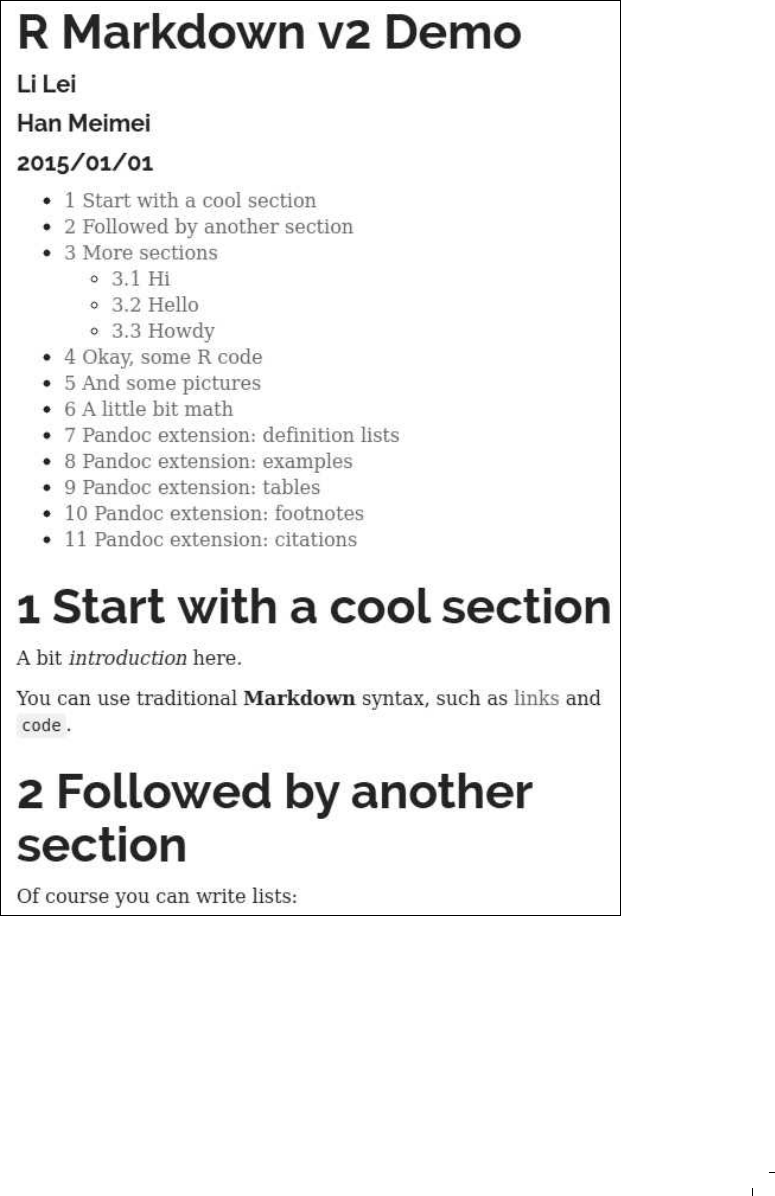
R Markdown 181
FIGURE 14.3: A preview of the “readable” theme (you can see the fonts
are different with Figure 14.1), with a table of contents and numbered
sections.

182 Dynamic Documents with R and knitr
Pandoc has an option to make the HTML file self-contained by em-
bedding all external dependencies into the HTML file. For example,
JavaScript files are read into the HTML file, and images are base64 en-
coded. You can share a self-contained HTML file just like a PDF file; ev-
erything you need has been embedded into a single file. In rmarkdown,
this is controlled by the option self_contained. When you have mul-
tiple Rmd files to be rendered by rmarkdown, it may be a good idea to
turn off the self-contained mode, otherwise there will be a lot of redun-
dancy since some external dependencies may be embedded into every
single HTML output file. When the self-contained mode is off, you can
put the shared dependencies into a common directory, specified via the
lib_dir option, e.g.,
---
output:
html_document:
self_contained: no
lib_dir: assets
---
Sometimes you may want to include additional content in the HTML
header, before the body, or after the body of the document. In these
cases, rmarkdown has an option includes in which you can specify
the filenames of the additional content. Suppose you want to use the
JavaScript library D3 (http://d3js.org) in the HTML output, then you
can write this in a file doc_header.html:
<script src="http://d3js.org/d3.v3.min.js" charset="utf-8">
</script>
You also have two files doc_before.html and doc_after.html, which
are the content to be inserted before and after the body, respectively. For
example, you may want to write a navigation menu in doc_before.html,
and some copyright information in doc_after.html. These three files can
be included in the HTML output file by:
---
output:
html_document:
includes:
in_header: doc_header.html
before_body: doc_before.html
after_body: doc_after.html
---

R Markdown 183
For any output format, Pandoc needs a template to create the output
file. There are several Pandoc variables available in the template, and
you can use these variables to define your own template. For example,
this can be a minimal HTML template:
<html>
<head>
<title>$title$</title>
</head>
<body>
$body$
</body>
</html>
We only used two variables $title$ and $body$ in this template.
The first variable contains the document title specified in the title
field in the YAML metadata. The second variable is the body of the
Markdown document after it is converted to HTML. You can learn
more possible variables from either the rmarkdown source package
(https://github.com/rstudio/rmarkdown) or Pandoc’s default tem-
plates (https://github.com/jgm/pandoc-templates).
To use a custom template, you can use the template field in YAML,
e.g.,
---
output:
html_document:
template: my_template.html
---
Finally, you can customize command-line arguments to be passed to
Pandoc in the pandoc_args field. As a matter of fact, the R arguments in
html_document() are eventually converted to Pandoc arguments. For ex-
ample, the R argument self_contained = TRUE (or self_contained:
yes in YAML) is equivalent to the Pandoc argument --self-contained,
and also equivalent to this in YAML:
---
output:
html_document:
pandoc_args: "--self-contained"
---

184 Dynamic Documents with R and knitr
So far we have covered most of the possibilities to customize the
output on the Pandoc’s Markdown side. It is also possible to customize
knitr chunk options in YAML. Currently there are four chunk options
that you can set in YAML:
fig_width, fig_height the default size of the figures
fig_retina a scaling ratio for Retina displays; the default is 2 in rmark-
down, which means a figure of the size m × n has an actual size of
2m ×2n, but is scaled to half of its actual size in the output (this can
improve the image qualities on Retina displays)
fig_caption whether to render and show figure captions (this basically
means the figure environment with \caption{} when the output
format is L
A
T
E
X); if FALSE, you will not see the figure caption in HTML
output, since the caption will be put in the alt attribute of the <img>
tag, which is invisible
Apparently, the fig_retina option will make the file size of images
larger in return for the image quality. You can try fig_retina = TRUE
and FALSE separately, and see if you can notice any differences on your
device.
14.3.2 L
A
T
E
X/PDF Document
Once you are familiar with the HTML document format, it will be easy
for you to master other output formats, because many options are com-
mon in these formats. For example, you can also use the options such
as fig_width, fig_height, toc, number_sections, and highlight in
pdf_document(). In this section, we only focus on the options that are
specific to PDF document output.
Figure 14.4 is a preview of a page in the PDF output from the same
example we used in the previous section. It does not look too much
different from Figure 14.2. For the same R Markdown document, ev-
erything that worked in the HTML output still works in L
A
T
E
X/PDF,
including section headings, tables, footnotes, and citations, etc.
Similarly, we can add a table of contents, and number the sections
as we did for the HTML output (Figure 14.5):
---
output:
pdf_document:
number_sections: yes
toc: yes
---

R Markdown 185
Pandoc extension: tables
A table here.
Table 1: Demonstration of simple table syntax.
Sepal.Length Sepal.Width Petal.Length Petal.Width Species
5.1 3.5 1.4 0.2 setosa
4.9 3.0 1.4 0.2 setosa
4.7 3.2 1.3 0.2 setosa
4.6 3.1 1.5 0.2 setosa
5.0 3.6 1.4 0.2 setosa
5.4 3.9 1.7 0.4 setosa
Pandoc extension: footnotes
We can also write footnotes
1
.
Or write some inline footnotes
2
.
Pandoc extension: citations
We compile the R Markdown file to Markdown through
knitr
(Xie 2014) in R
(R Core Team 2014). For more about Xie (2014), see http://yihui.name/knitr.
References
R Core Team. 2014. R: A Language and Environment for Statistical Computing.
Vienna, Austria: R Foundation for Statistical Computing. http://www.R-project.
org/.
Xie, Yihui. 2014. Knitr: A General-Purpose Package for Dynamic Report
Generation in R. http://yihui.name/knitr/.
1
hi, I’m a footnote
2
as you can see here
4
FIGURE 14.4: A preview of the 4th page of the PDF output document
from the R Markdown v2 example.

186 Dynamic Documents with R and knitr
R Markdown v2 Demo
Li Lei Han Meimei
2015/01/01
Contents
1 Start with a cool section 2
2 Followed by another section 2
3 More sections 2
3.1 Hi . . . . . . . . . . . . . . . . . . . . . . . . . . . . . . . . . . . 2
3.2 Hello . . . . . . . . . . . . . . . . . . . . . . . . . . . . . . . . . . 2
3.3 Howdy . . . . . . . . . . . . . . . . . . . . . . . . . . . . . . . . . 2
4 Okay, some R code 3
5 And some pictures 3
6 A little bit math 4
7 Pandoc extension: definition lists 4
8 Pandoc extension: examples 4
9 Pandoc extension: tables 5
10 Pandoc extension: footnotes 5
11 Pandoc extension: citations 5
References 5
1
FIGURE 14.5: A preview of the PDF output document, with a table of
contents and numbered sections.

R Markdown 187
Pandoc has a few L
A
T
E
X-specific options that you can use in the YAML
metadata, and you can find the full documentation on the Pandoc web-
site. We only list a few of them here:
fontsize the font size of the document, e.g., 10pt, 11pt, 12pt
documentclass the document class, e.g., article, book, report
classoption options for the document class, e.g., a4paper, twocolumn
geometry options for the geometry package, e.g., tmargin=2cm, bmar-
gin=2cm, lmargin=3cm, rmargin=3cm
Note these are top-level options in YAML, and you should not put them
under the pdf_document field.
The default L
A
T
E
X engine is pdflatex, and you can change it via the
latex_engine option in pdf_document(). Currently possible engines are
pdflatex, xelatex, and lualatex. You may also preserve the interme-
diate L
A
T
E
X output file via the keep_tex option, which can be useful for
debugging and other purposes.
Below is an example of the YAML metadata for a document that
uses the book class, a font size of 11pt, a two-column layout, custom
margin settings, the XeL
A
T
E
X engine, and also preserves the L
A
T
E
X file:
---
documentclass: book
classoption: twocolumn
fontsize: 11pt
geometry:
- tmargin=2cm
- bmargin=2cm
- lmargin=3cm
- rmargin=3cm
output:
pdf_document:
latex_engine: xelatex
keep_tex: yes
---
We have introduced the includes and template options in the pre-
vious section, and they may be more useful for L
A
T
E
X output, because
it is very common for L
A
T
E
X users to customize the output using cer-
tain L
A
T
E
X packages in the preamble. You can put such content in an
external file, and include it in the preamble via the in_header option
under the includes option. If you are not satisfied with the default

188 Dynamic Documents with R and knitr
L
A
T
E
X template, you can just write your own. Before you really do it,
please check the Pandoc documentation carefully to see if you can get
what you want by YAML options. It is relatively easy to write a new
L
A
T
E
X template, but it may not be trivial to maintain it in the future,
since you need to be aware of possible future changes in Pandoc.
14.3.3 Word Document
There are not many options to customize for Word documents. You can
still set the figure size, and syntax highlighting themes, etc. Figure 14.6
shows the Word output from the example in Microsoft Word 2013.
The most important and useful feature for Word documents is per-
haps the template. For other document formats, you can provide a
plain text template, but you cannot easily do so for Word, because a
Word document is a relatively complicated binary file. However, Pan-
doc allows you to provide a Word document as its “reference docu-
ment,” which is essentially a style template. This reference document
must be based on one of Pandoc’s Word output documents, in which
you update its styles for different elements. Note only the styles defined
in the document will be used, and the content will be largely ignored.
We have prepared a short video at https://vimeo.com/110804387
to show you how to define styles in Word documents. You can also see
Figure 14.7 and 14.8. The basic steps are:
1. Create an arbitrary Word document using Pandoc, e.g., use
word_document as the output option in the YAML metadata;
2. Open the Word document, and find the “Styles” panel indi-
cated in Figure 14.7;
3. Put the cursor on the element of which you want to mod-
ify the style, and there should be an item in the Styles panel
highlighted;
4. Open the item by clicking the ¶ symbol on the right, and you
will see a window like Figure 14.8. That is where you can
modify the styles. For example, you can change the font fam-
ily of the title element to be Bookman Old Style.
After you update the styles of this Word document, you can save it
(say, as template.docx under the same directory as the Rmd file) and use
it as the reference document:
---
output:
word_document:

R Markdown 189
FIGURE 14.6: A preview of the Microsoft Word (2013) document from
R Markdown v2.
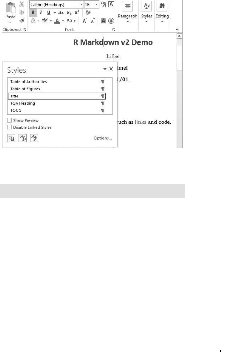
190 Dynamic Documents with R and knitr
FIGURE 14.7: Open the styles panel in Word: find a pane named
“Styles” on the toolbar, and expand it to a floating panel.
renference_docx: template.docx
---
Besides the styles of the elements, the styles of the layout can also
be respected if you use Pandoc >= 1.13. For example, the margins, page
size, page orientation, header, and footer in the reference document will
be carried over to the new Word document.
14.3.4 Markdown Documents
An R Markdown document can be converted to different flavors of
Markdown documents, such as Pandoc’s Markdown, the original (strict)
Markdown, Github Flavored Markdown, MultiMarkdown, and PHP
Markdown Extra. You can use the function md_document() for render()
or output: md_document in YAML. The main option for md_document
is variant, which specified which flavor of Markdown you want.

R Markdown 191
FIGURE 14.8: Modify styles of elements in Word: you can change the
font family, font size, font style, and color, etc.
14.3.5 ioslides Presentation
R Markdown can be used to create slides for presentation purposes.
With the process of Web technologies, HTML5 slides seem to be pop-
ular nowadays. You can present slides in a Web browser. This is con-
venient since you do not need special software packages to display the
slides, and you can find a Web browser almost everywhere. This is not
true for proprietary software such as Microsoft PowerPoint or Keynote
for Mac.
There are two types of built-in HTML5 presentation formats in rmark-
down: ioslides and Slidy. You can extend rmarkdown to use your own
favorite HTML5 presentation library.
For ioslides, each first-level section heading will create a separate

192 Dynamic Documents with R and knitr
FIGURE 14.9: The title slide of an ioslides presentation: you can also
use the table of contents in RStudio to navigate through the slides.
slide with a dark background by default; each second-level heading cre-
ates a new slide with the content of this section on it. If you do not want
a section heading, you can create a new slide with three dashes ---.
Figure 14.9 is a screenshot of ioslides in the RStudio preview window,
created using the same example as previous sections and the YAML
metadata (if you really try this example, you may want to remove the
content between the first-level heading and second-level heading):
---
output:
ioslides_presentation: default
---
When you do the presentation, you may want to use the fullscreen
mode, which can be turned on by the keyboard shortcut f (just press

R Markdown 193
the F key). The key W toggles the widescreen mode. If the slide size is
too big or too small, you can zoom in/out the page. Normally you can
do it by holding the Ctrl (or Command) key, then press Plus (+) or Minus
(-).
There are a few options for the ioslides_presentation format you
can use to tweak the appearance of the slides:
incremental (yes/no) whether to show bullets incrementally
logo an image that you want to use as the logo in the slides (it will be
displayed in the footer of each slide)
css a custom CSS file
You can also customize each slide individually. For example, if you put
a token {.build} after a second-level section heading, the elements on
this page will be displayed incrementally as you proceed in the presen-
tation, e.g.,
## A new slide {.build}
First show this.
Then show that.
Finally show a funny GIF animation.

HTML5 slides are usually for presentation instead of printing pur-
poses. However, you may also print the slides as PDFs from your Web
browser. At the moment, we recommend you to use Google Chrome
if you want to print the slides. You should expect the appearance of
printed slides to differ from that of the displayed slides.
14.3.6 Slidy Presentation
The rules of writing slides for Slidy are the same as ioslides. The func-
tion for Slidy presentation output in rmarkdown is slidy_presentation().
Figure 14.10 shows one slide of the Slidy presentation created from the
R Markdown example.
A few keyboard shortcuts are available, e.g., press C to see the table
of contents, S to make the font smaller, and B to make the font bigger,
etc.
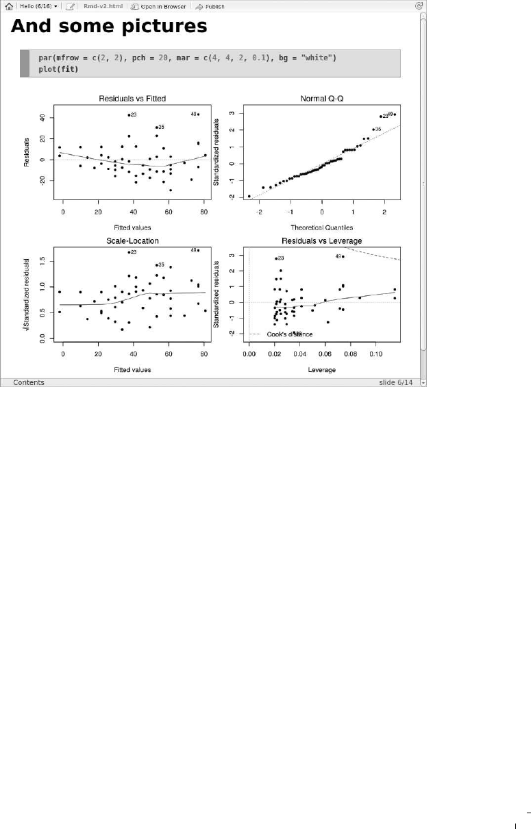
194 Dynamic Documents with R and knitr
FIGURE 14.10: One slide from the Slidy presentation generated from
the R Markdown example: you can also click “Contents” at the bottom
to show the table of contents.
Besides the incremental and css options we mentioned before, Slidy
has some additional features that may be useful, including the options:
duration sets a countdown timer in the footer to remind you of the
time, e.g., if you have a 50-minute talk, you can set duration: 50
in YAML
footer a custom message in the footer, e.g., you can display the name
of your institute or copyright information
To print Slidy slides, you can also use Google Chrome.
14.3.7 Beamer Presentation
Beamer, introduced in Section 12.3.4 is a L
A
T
E
X application, so you can
build an Rnw file as a L
A
T
E
X document with code chunks shown in Sec-

R Markdown 195
tion 12.3.4 and compile directly into the PDF format. Markdown is sim-
pler and faster for all but veteran L
A
T
E
X users, so we recommend trying
it with the beamer_presentation format. If you need some of the more
advanced Beamer or L
A
T
E
X features, they can be added within Mark-
down as Pandoc supports L
A
T
E
X code within Markdown.
Figure 14.11 shows two slides of the Beamer presentation created
from the previous R Markdown example. All we did was change the
YAML metadata to:
---
title: "R Markdown v2 Demo"
author:
- Li Lei
- Han Meimei
date: "2015/01/01"
output:
beamer_presentation:
theme: AnnArbor
bibliography: Rmd-v2.bib
---
If we were to write the slides in raw L
A
T
E
X, the source document
would be like this:
\documentclass{beamer}
\usetheme{AnnArbor}
\title{R Markdown v2 Demo}
\author{Li Lei \and Han Meimei}
\date{2015/01/01}
\begin{document}
\frame{\titlepage}
\begin{frame}{Start with a cool section}
A bit \emph{introduction} here.
You can use traditional \textbf{Markdown} syntax, such as
\href{http://yihui.name/knitr}{links} and \texttt{code}.
\end{frame}
\begin{frame}{Followed by another section}

196 Dynamic Documents with R and knitr
R Markdown v2 Demo
Li Lei Han Meimei
2015/01/01
Li Lei, Han Meimei R Markdown v2 Demo 2015/01/01 1 / 13
Pandoc extension: examples
We have some examples.
1
Think what is 0.3 + 0.4 - 0.7. Zero. Easy.
2
Now think what is 0.3 - 0.7 + 0.4. Still zero?
People are often surprised by (2).
Li Lei, Han Meimei R Markdown v2 Demo 2015/01/01 9 / 13
FIGURE 14.11: Two slides from the Beamer presentation created by R
Markdown: the title slide, and the slide that shows the Pandoc exten-
sion of the example environment.

R Markdown 197
Of course you can write lists:
\begin{itemize}
\item
apple
\item
pear
\item
banana
\end{itemize}
....
\end{document}
Compare that with the R Markdown source code in Section 14.3.1,
and hopefully you see how much more code you would have to type
when writing in raw L
A
T
E
X than writing in Markdown.
Each new slide is a new section in Markdown, and the level of the
section is determined by the highest level in the document hierarchy
that is followed immediately by the slide content. In the following ex-
ample, each first-level section (#) is a new slide:
---
output: beamer_presentation
---
# One Section
- content
- content
# Another Section

And in this example, each sub-section (##) is a new slide:
---
output: beamer_presentation
---
# One Section

198 Dynamic Documents with R and knitr
## One Sub-section
- content
- content
# Another Section
## Another Sub-section

To display list items incrementally, you can use the incremental op-
tion just like what we can do for ioslides and Slidy presentations. Other
options such as toc, highlight, fig_width, fig_height, fig_caption,
includes, and template have been explained in previous sections.
There are many themes (including font themes and color themes) in
Beamer. You can use them via the theme, fonttheme, and colortheme
options. Figure 14.11 used the AnnArbor theme, and default font/color
themes. If you use RStudio, you can choose these themes from the GUI,
so you do not need to remember the many theme names.
14.3.8 Other Formats
Besides the document and presentation formats, rmarkdown also has
two special output formats: html_vignette() for HTML package vignettes
(Section 15.4) and tufte_handout() for the Tufte handout (here Tufte refers
to Edward R. Tufte).
The html_vignette() format is a wrapper of html_document(), with a
special CSS theme; the file size of the HTML vignette produced by
html_document() is too big because it contains the Twitter Bootstrap as-
sets, the jQuery library, and highlight.js by default. The html_vignette()
format has removed all these components, and uses a single lightweight
CSS file. The option fig_retina has been set to 1 to further reduce
the image file sizes. This format function is a good example of how
to build your own format based on existing format functions, and its
source code is very simple:
html_vignette <- function(fig_width = 3,
fig_height = 3, dev = "png", css = NULL,
...) {
if (is.null(css)) {
css <- system.file("rmarkdown", "templates",

R Markdown 199
"html_vignette", "resources",
"vignette.css", package = "rmarkdown")
}
html_document(fig_width = fig_width,
fig_height = fig_height, dev = dev,
fig_retina = FALSE, css = css, theme = NULL,
highlight = "pygments", ...)
}
The tufte_handout() format is a wrapper for the L
A
T
E
X document class
tufte-handout.cls. The most notable characteristics of the Tufte handout
style are perhaps the use of sidenotes, and the well-designed typogra-
phy. See Figure 14.12 for an example page. Its YAML metadata is this:
---
title: "Tufte Handout"
author: "John Smith"
date: "August 13th, 2014"
output: rmarkdown::tufte_handout
---
14.4 Interactive Documents with Shiny
Shiny (Chang et al., 2015) is a Web application framework that makes
it easy to create interactive apps using R. You can create a Web user in-
terface (UI) using Shiny UI functions, e.g., text input boxes, drop-down
lists, radio buttons, and sliders, etc. These UI elements can interact with
R after you specify the server logic in R, e.g., after you click a button,
what you expect R to do. If you are not familiar with Shiny, please
check out the website http://shiny.rstudio.com to learn the basics
about Shiny.
Because a Shiny app is basically an HTML page, and it happens that
R Markdown can be rendered to HTML, too, it is possible to combine
R Markdown and Shiny in one document. We call such documents “in-
teractive documents,” since they contain interactive components from
Shiny. Figure 14.13 shows a minimal example of an interactive docu-
ment. Its source document is as follows:
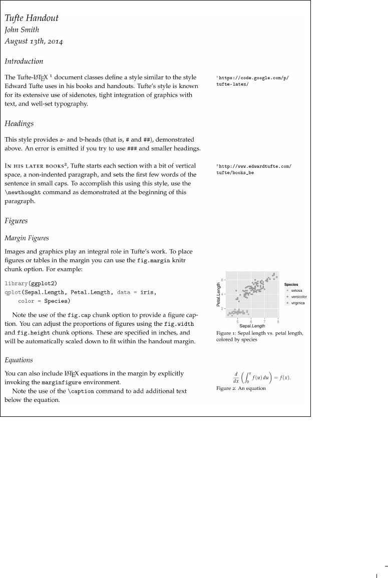
200 Dynamic Documents with R and knitr
FIGURE 14.12: An example page using the Tufte handout style: you
can arrange elements into the side margin, such as footnotes, figures,
equations, and so on.

R Markdown 201
FIGURE 14.13: A simple interactive document using R Markdown and
Shiny: you can change the value of the slider, and the number of bins
in the histogram will be automatically changed.

202 Dynamic Documents with R and knitr
---
title: "R Markdown v2 Demo"
runtime: shiny
output: html_document
---
```{r}
library(shiny)
sliderInput("bins", "Number of bins:", min = 1, max = 50,
value = 30)
renderPlot({
x <- faithful[, 2] # Old Faithful Geyser data
bins <- seq(min(x), max(x), length.out = input$bins + 1)
# draw the histogram with the specified number of bins
hist(x, breaks = bins, col = 'darkgray', border = 'white')
})
```
To turn a normal R Markdown document into an interactive docu-
ment, you only need to add the option runtime: shiny in the YAML
metadata. Then you can use functions in the shiny package. In the
above example, we created a slider on the HTML page using sliderIn-
put(), which is a UI function in shiny. The id of the slider is bins. Then
we rendered a histogram using the renderPlot() function. The most im-
portant bit in this code chunk is input$bins, which is a variable value
associated with the slider with the id bins. When we update the value
of the slider, its value will be passed to the expression in renderPlot(),
and the plot will be redrawn accordingly.
Instead of render(), interactive documents should be compiled by the
run() function in rmarkdown. If you use RStudio, you will see that the
label of Knit button on the toolbar becomes Run Document after you add
runtime: shiny to an R Markdown document, and you can click the
button to run the document.
Not all Shiny apps can be so simple as the one in Figure 14.13. When
you have several UI elements, you may want to arrange them in a sepa-
rate app instead of writing them out in code chunks linearly. The func-
tion shinyApp() in shiny allows you to build a full app by specifying all
UI elements and the server logic in one function. Then you can either
embed full apps using shinyApp() explicitly in R Markdown, or write
your own function that returns a shinyApp() object, so that other people
can easily use your app as well.
Static HTML documents can be uploaded to any website or emailed

R Markdown 203
when you want to share them. For interactive documents, there must be
an active R session running behind them. One possible way to share in-
teractive documents is to publish them to http://shinyapps.io, which
is hosted by RStudio. If you do not want to publish to this website, you
can set up your own Shiny Server: http://www.rstudio.com/products/
shiny/shiny-server/.
14.5 Extending R Markdown v2
If none of the output format functions meet your need, you can extend
them or write a completely new format. Before you do it, please make
sure you have looked at all the possibilities in the existing output for-
mats. Sometimes there is no need to invent anything new. For example,
if all you want is to use a different L
A
T
E
X document class, you may as
well set the documentclass option in the YAML metadata, although
you can certainly also write a new template with the desired document
class. Take the Tufte handout as an example:
---
title: "R Markdown v2 Demo"
author: John Smith
date: "2015/01/01"
output: pdf_document
documentclass: tufte-handout
classoption: nohyper
geometry: no
---
The above YAML metadata makes use of the existing pdf_document()
format. Alternatively, you can prepare a template like:
\documentclass{tufte-handout}
$if(title)$
\title{$title$}
$endif$
$if(author)$
\author{$for(author)$$author$$sep$ \and $endfor$}
$endif$
$if(date)$
\date{$date$}

204 Dynamic Documents with R and knitr
$endif$
\begin{document}
$if(title)$
\maketitle
$endif$
$body$
\end{document}
Then use the template option in pdf_document. There are a number
of disadvantages of writing a custom template like that:
• Pandoc’s default L
A
T
E
X is much more flexible (https://github.com/
jgm/pandoc-templates), which can also deal with the table of con-
tents, the list of figures, and the abstract, etc.;
• It requires more work to write a new template than to use existing
options in YAML;
• After you write a template, you will have to watch out for future
changes in Pandoc, which may break your template, or you may miss
some useful new features. By comparison, if you use Pandoc’s tem-
plates, you do not need to maintain them.
Then you may ask why we have the tufte_handout() format in rmark-
down after all. Actually what this new format does is more than just a
L
A
T
E
X template: it also defines a few knitr chunk options to produce full-
width figures (fig.fullwidth = TRUE) and margin figures (fig.margin
= TRUE). Existing output formats do not provide these two different fig-
ure types.
14.5.1 Templates
The first type of rmarkdown extension is to define a new template. We
have shown an example above for the Tufte handout, and also an ex-
ample earlier in Section 14.3.1 for HTML document output.
The repository https://github.com/jgm/pandoc-templates con-
tains all templates used by Pandoc, and you can also take a look at
the custom templates in the rmarkdown source package at https://
github.com/rstudio/rmarkdown. If there are any template variables
that you do not understand, you can check out the documentation at
http://johnmacfarlane.net/pandoc/.

R Markdown 205
To share a template with other users, the easiest way is to put it
in an R package under the inst/rmarkdown/templates/ directory. You
can create a new directory, say, my_template, and put the template file
under it. Your template may require certain dependencies, such as
CSS/JavaScript files, or L
A
T
E
X packages. They can be collected under
a sub-directory skeleton/ under my_template. In the skeleton/ directory,
you can also provide a sample Rmd file skeleton.Rmd. Finally, you can
describe the template in a YAML file template.yaml under my_template
with three YAML fields:
name the name of the template, e.g., “Journal of Statistical Software”;
description a short description of the template, e.g., “This is a template
for JSS articles”;
create_dir yes or no, or true or false (to be explained soon);
Suppose you installed such an R package named myPackage, then you
can create a new draft from the template using the draft() function:
rmarkdown::draft("my_article.Rmd", template = "my_template",
package = "myPackage")
This function looks for the template my_template in myPackage,
copies skeleton.Rmd as my_article.Rmd to the current working directory,
and also copies the dependencies. The YAML option create_dir men-
tioned above determines whether to create a new directory for the draft
my_article.Rmd.
RStudio has made this process even easier. From the menu File .
New File . R Markdown, you can see all templates in all locally installed
packages (Figure 14.14).
The rticles package (https://github.com/rstudio/rticles) is a
collection of templates for several L
A
T
E
X document classes. You can use
its templates to write papers in R Markdown for the Journal of Statistical
Software, and The R Journal, etc.
14.5.2 New Formats
The second type of rmarkdown extension is new output formats. The
new format can be based on an existing output format, or a completely
new format. The former is easy: you just define an R function that
returns an output format object, with certain options modified from
an existing output format function. As a minimal example, we create a
function html_toc below, turning the default value of the toc argument
from FALSE to TRUE:

206 Dynamic Documents with R and knitr
FIGURE 14.14: Create a new R Markdown document from templates:
you can select a template from the list.
html_toc <- function(toc = TRUE, ...) {
rmarkdown::html_document(toc = toc, ...)
}
A new format function should be put in an R package (we still as-
sume its name is myPackage), and then you can use it in YAML. Here
are two examples:
---
output: myPackage::html_toc
---
---
output:
myPackage::html_toc:
toc: no
self_contained: no
---
R Markdown 207
FIGURE 14.15: Create an E-book from R Markdown: this figure shows
the title page of the EPUB book in FBReader (a free E-book reader).
For the second example, what will be called when we render this
Rmd file is:
rmarkdown::render("foo.Rmd", myPackage::html_doc(toc = FALSE,
self_contained = FALSE))
# which is essentially render('foo.Rmd',
# html_document(toc = FALSE, self_contained = FALSE))
As we explained in Section 14.3.1, the output format is a list of three
types of options: knitr options, Pandoc options, and rmarkdown op-
tions. We customized the Pandoc toc in the above minimal example,
and you can certainly customize more options in the output format
function. There are a few helper functions output_format(), knitr_options(),
and pandoc_options() in rmarkdown that you can use to compose the
output format. See the repository https://github.com/jjallaire/
revealjs for an example of how to create a new format for reveal.js
(an HTML5 presentation format). Below we show a minimal example
of how to create an output for EPUB (an E-book format):
#' @importFrom rmarkdown output_format
#' @importFrom rmarkdown knitr_options
#' @importFrom rmarkdown pandoc_options
epub_book <- function(to = c("epub", "epub3")) {
to <- match.arg(to)
optk <- knitr_options()
optp <- pandoc_options(to, ext = ".epub")
output_format(knitr = optk, pandoc = optp)
}

208 Dynamic Documents with R and knitr
Put this function in the package myPackage, and you will be able
to create E-books from R Markdown. Here is a minimal R Markdown
example (Figure 14.15):
---
title: "R Markdown v2 Demo"
author:
- Li Lei
- Han Meimei
date: "2015/01/01"
output: myPackage::epub_book
---
# Start with a cool section
```{r}
1 + 1
```
The key in the format function epub_book() was to specify the argu-
ment to of pandoc_options() to be either epub or epub3. Pandoc supports
a large number of document formats, and rmarkdown only included a
small subset of them. You can build your own format function using
the approach introduced above.
14.5.3 HTML Widgets
We explained the includes option in the YAML metadata in Section
14.3.1. When you want to include JavaScript libraries in the HTML
document output, you can use the includes option. There are two dis-
advantages of this approach:
1. It is not portable, in the sense that when you share the R
Markdown document with other people, you should remem-
ber to copy the dependencies specified in the includes op-
tion; it is not convenient for other people to reuse your de-
pendencies, either;
2. You have to write (sometimes a lot of) JavaScript code in R
Markdown to call the JavaScript libraries, but not all R users
are familiar with JavaScript, so they may not be able to work
on the R Markdown document.
The idea of HTML widgets is to provide native R interfaces to JavaScript
libraries, so that even those who do not understand JavaScript can still

R Markdown 209
use the libraries without worrying about the underlying dependencies
or JavaScript syntax. When you draw a plot using a JavaScript library,
all you need to do is call an R function in a code chunk.
The htmlwidgets package (Vaidyanathan et al., 2014) was designed
for package developers to port JavaScript libraries into R easily. It is
well-documented at http://www.htmlwidgets.org, and you can see
several example packages on the website, too. We will not describe
the technical details here, and we just show a quick example of what an
HTML widget looks like. Here is a minimal R Markdown example (you
need to install the DT package from https://github.com/rstudio/DT
before trying this example):
---
title: "R Markdown v2 Demo"
author:
- Li Lei
- Han Meimei
date: "2015/01/01"
output: html_document
---
Here is a table generated by the DataTables library.
```{r}
DT::datatable(iris)
```
Figure 14.16 shows the output. The DT package is an interface to
the JavaScript library DataTables (http://datatables.net). As you
can see, the R Markdown source document is really simple, and you
do not see the JavaScript files or any JavaScript code at all. You simply
call the function datatable(), and your data frame will be displayed via
DataTables. The hard work of passing data to the HTML page, parsing
and rendering it has been done by the package authors, and users do
not have to understand all the underlying technical details.
14.6 Changes in R Markdown from v1 to v2
If you happen to have started using R Markdown when it was v1, here
is a list of changes that you should be aware of when you transition
from v1 to v2:

210 Dynamic Documents with R and knitr
FIGURE 14.16: A table created by the DataTables library in R Mark-
down: you can order the columns, search in the table, and the full table
can be displayed on multiple pages.

R Markdown 211
• The knitr package is no longer loaded (strictly speaking, attached) by
default in v2, which means the functions and objects in the knitr pack-
age are not available unless you explicitly load the package, e.g., via
the command library(knitr); otherwise, you may get errors like
“object ’opts_chunk’ not found”;
• The chunk options fig.path (figure path) and cache.path (cache path)
are modified in rmarkdown when rendering an Rmd file. In knitr,
they are figure/ and cache/, respectively. Now in rmarkdown, they
are foo_files/figure-format/ and foo_files/cache-format/, re-
spectively, where foo is the base filename of the input Rmd file with-
out the file extension, and format is the output format, e.g., tex or
html;
• The chunk option error was changed from TRUE to FALSE, and the
implication is that R will stop by default, instead of showing the error
messages in the R Markdown output document (see Section 6.2.4);
• The chunk options fig.width, fig.height, and fig.retina may take
different values, depending on the output format. You can either
check the rmarkdown documentation of output format functions, or
print str(knitr::opts_chunk$get()) in your R Markdown docu-
ment to see the values of chunk options.


15
Applications
So far we have been introducing the usage of knitr with short examples
for the sake of simplicity. In this chapter we use some concrete and
complete examples to show how knitr works with real applications;
we do not explain every single detail of these applications, and we only
point out the critical parts in them.
15.1 Homework
For homework applications, R Markdown might be the preferred doc-
ument format to work with due to its simplicity, and homework is usu-
ally not targeted at publication. As mentioned before, RPubs (http:
//rpubs.com) is a platform for sharing (HTML) reports generated from
RStudio by knitr. There are many homework submissions, too.
Since a homework report is relatively simple, we may not need too
many knitr features; some common features used in homework are:
set the size of plots (fig.width and fig.height), hide the source code
because the grader may not wish to read it (echo = FALSE), and enable
cache for time-consuming computing jobs (cache = TRUE), etc. Other
features that come by default such as tidy = TRUE and highlight =
TRUE can help users who do not care about coding styles produce more
readable code in the output document.
Now we show an example of Gibbs sampling. For the bivariate Nor-
mal distribution
X
Y
∼ N
µ
X
µ
Y
,
σ
2
X
ρσ
X
σ
Y
ρσ
X
σ
Y
σ
2
Y
(15.1)
we know the conditional distributions
Y|X = x ∼ N
µ
Y
+
σ
Y
σ
X
ρ(x − µ
X
), (1 −ρ
2
)σ
2
Y
X|Y = y ∼ N
µ
X
+
σ
X
σ
Y
ρ(y −µ
Y
), (1 −ρ
2
)σ
2
X
(15.2)
213

214 Dynamic Documents with R and knitr
so we can use the Gibbs sampling to generate random numbers from
the joint Normal distribution. First we initialize x
(0)
and y
(0)
, then re-
peatedly generate x
(k)
∼ f (x|y
(k−1)
) and y
(k)
∼ f ( y|x
(k)
). The R code
below is a translation of 15.2:
rbinormal <- function(n, mu1, mu2, sigma1, sigma2, rho) {
# initialize
x <- rnorm(1, mu1, sigma1)
y <- rnorm(1, mu2, sigma2)
xy <- matrix(nrow = n, ncol = 2, dimnames = list(NULL,
c("X", "Y")))
# sample from conditional distributions
for (i in 1:n) {
x <- rnorm(1, mu1 + sigma1/sigma2 * rho * (y - mu2),
sqrt(1 - rho^2) * sigma1)
y <- rnorm(1, mu2 + sigma2/sigma1 * rho * (x - mu1),
sqrt(1 - rho^2) * sigma2)
xy[i, ] <- c(x, y)
}
xy
}
Figure 15.1 shows the first 20 steps of Gibbs sampling for the bivari-
ate Normal distribution with µ
X
= 0, σ
X
= 2, µ
Y
= 1, σ
Y
= 3, ρ = 0.7.
set.seed(123)
n <- 20
z <- rbinormal(n, mu1 = 0, mu2 = 1, sigma1 = 2, sigma2 = 3,
rho = 0.7)
plot(z, pch = 19)
arrows(z[-n, 1], z[-n, 2], z[-1, 1], z[-1, 2], length = 0.15,
col = "gray40")
And we can draw some samples as well:
z <- rbinormal(5000, 0, 1, 2, 3, 0.7)
smoothScatter(z, nbin = 64)
points(0, 1, col = "white", pch = 19) # theoretical mean
Figure 15.2 shows 5,000 samples from this distribution, and we can
calculate the sample means, standard deviations, and the correlation,
which should be close to the corresponding theoretical values:

Applications 215
-3 -2 -1 0 1 2 3
-6
-4
-2
0
2
4
6
X
Y
FIGURE 15.1: Trace of Gibbs sampling for a bivariate Normal distribu-
tion: the arrows show the first 20 steps of Gibbs sampling.
-6 -4 -2 0 2 4 6
-5
0
5
10
X
Y
FIGURE 15.2: 5000 points from Gibbs sampling: the smoothed scatter-
plot shows the density of the 2D distribution.

216 Dynamic Documents with R and knitr
apply(z, 2, mean) # sample mean
## X Y
## 0.001287 0.971010
apply(z, 2, sd) # sample sd
## X Y
## 1.973 2.971
cor(z) # sample correlation
## X Y
## X 1.0000 0.6948
## Y 0.6948 1.0000
In this small application, we used cache (although this particular
example is not too slow) and TikZ graphics. We adjusted the plot sizes
(5 ×3 for Figure 15.1 and 5 ×4 for Figure 15.2). Note the narratives and
code chunks are interwoven, and the reader can learn the theory, see
the computing, and verify the results in the same report. Everything
is transparent, and it will be easy to find out errors. Sometimes the
computer code we write may not really reflect what we said in theory,
and it will be hard to find out such errors if we separate computing
from reporting.
In terms of data, code and software sharing, we cannot
yet rely on goodwill and self discipline when it comes to
sharing publication material and making studies fully re-
producible.
Huang and Gottardo (2013)
Comparability and reproducibility of biomedical data
People have been proposing sharing data, code, and software in
data analysis for the sake of reproducible research, e.g., Huang and
Gottardo (2013). We believe that more efforts in education should be
an important step, and we can start with reproducible homework.

Applications 217
15.2 Serve Dynamic Documents
The servr package (Xie, 2015c) provides some simple HTTP server func-
tions to serve files under a given directory based on the httpuv package.
To some degree, this package is like python -m SimpleHTTPServer or
python -m http.server if you are familiar with Python. Originally it
was designed to serve static files under a directory, and the main func-
tion was httd():
servr::httd("./")
If you run the above function in the R console, R will launch your
Web browser to show a list of files under the current working directory
(./), or show index.html if this file exists. You can click the links on the
files to view their content.
Later servr was extended based on knitr and rmarkdown, so it
can also serve dynamic R Markdown documents. There are functions
jekyll(), rmdv1(), and rmdv2() in this package to serve HTML files gener-
ated from R Markdown documents (via knitr or rmarkdown). R Mark-
down documents can be automatically recompiled when their HTML
output files are older than the corresponding source files, and HTML
pages in the Web browser can be automatically refreshed accordingly,
so you can focus on writing R Markdown documents, and results will
be updated on the fly in the Web browser. This saves you two steps:
click the Knit HTML button, and refresh the Web browser. Both steps
can be distracting when you write a report. With servr, all you need to
do is write the R Markdown document after you launch a server.
This is even more useful when you write R Markdown documents
in the RStudio IDE, because servr has set the Web browser to be the
RStudio Viewer by default when it detects the RStudio IDE, and you
can put the source document and its output side by side like the layout
in Figure 15.3. It is completely fine if you do not use RStudio — the
automatic compilation and refreshing also work if you use other editors
and Web browsers.
The functions rmdv1() and rmdv2() correspond to R Markdown v1
and v2, respectively. After you call servr::rmdv1() or servr::rmdv2()
in the R console, you can click the HTML file foo.html if it has its source
document foo.Rmd, and view the HTML output. Then whenever you
edit foo.Rmd and save it, servr will automatically recompile it and re-
fresh the HTML output page.
The function jekyll() is like rmdv1() and rmdv2(), but is tailored for
Jekyll websites. We have briefly introduced Jekyll in Section 13.4. It

218 Dynamic Documents with R and knitr
FIGURE 15.3: The layout of an R Markdown document (top-left panel)
and its output in the RStudio Viewer (right panel): we typed a servr
function in the R console (bottom-left), and the output of the R Mark-
down is showed in the RStudio Viewer. This figure is only for illustra-
tion purposes; see https://github.com/yihui/servr for the original
image if you want to read the text in it.
is tedious to compile R Markdown posts or pages to Markdown again
and again, and that is why jekyll() can be useful. Once you call the
function servr::jekyll() in the root directory of a Jekyll website, you
will get a preview of the website in your Web browser. Besides, as
you edit and save your blog post, the Web browser will refresh the
page to show the updated output. The knitr-jekyll repository (https:
//github.com/yihui/knitr-jekyll) is an example of serving Jekyll
websites using servr.
Later we will introduce package vignettes in Section 15.4, and the
function vign() in servr can be used to serve HTML vignettes while
we develop an R package. Its advantage is that it does not preserve
the HTML output file in the source package when serving the vignette,
which makes the source package clean.
For those who are curious about the technical details, the implemen-
tation is based on WebSockets. When servr shows an HTML page, it
also injects a piece of JavaScript code in it to set up a WebSocket connec-
tion to talk to R periodically (e.g., on one-second basis). Every time R
receives a request from the WebSocket, it will compare the timestamps
of Rmd files with their output HTML files. If an Rmd file is newer
than its HTML output, servr will call knitr or rmarkdown to recom-
pile the Rmd file to HTML, then send a message back to the WebSocket.

Applications 219
all: example.html
%.html: %.Rmd
Rscript -e "rmarkdown::render('$^')"
FIGURE 15.4: A Makefile example for the function make() in servr: the
HTML file to be generated is specified in the target all, and a rule is
specified on how to generate an HTML file from an Rmd file via rmark-
down.
When the WebSocket receives this message, it calls location.reload()
in JavaScript to refresh the page.
A critical step in this process is to check if we need to recompile
any Rmd files. This is a task that GNU Make (http://www.gnu.org/
software/make/) is good at, so servr also provided a function make()
so that you can provide your own Makefile to rebuild Rmd files when
necessary. Figure 15.4 is an example Makefile for the make() function.
By default, a server function will block the current R session, which
can be a problem if you want to continue working in the same R ses-
sion. To solve this problem, you can use the argument daemon = TRUE
for the server function, e.g., httd(daemon = TRUE), or rmdv2(daemon =
TRUE). This tells servr to launch a daemonized server that will not block
the current R session.
15.3 Website and Blogging
We introduce a few websites and blogs built upon knitr in this section,
and the Web pages are created from either R Markdown or R HTML.
15.3.1 Vistat and Rcpp Gallery
Vistat (http://vis.supstat.com) is a website based on R Markdown
and Jekyll (Section 13.4). It aims to provide a gallery of reproducible
statistical graphics. The repository for the website is publicly available
on Github: https://github.com/supstat/vistat.
The core of this repository is the R script ./_bin/knit, which sets
some global chunk options and compiles Rmd documents to Mark-
down output. Math equations are rendered by MathJax, animations

220 Dynamic Documents with R and knitr
are supported through the SciAnimator library (Section 7.3.1), and we
can also create Web graphics via the D3 library.
After knitr has compiled Rmd source files to Markdown files, Jekyll
can compile Markdown to HTML, which gives us a website.
The Rcpp Gallery (http://gallery.rcpp.org) is a website for Rcpp
(Eddelbuettel et al., 2015) articles and examples, and it is also built on
R Markdown; in particular, it uses knitr’s Rcpp engine (Section 11.2.1).
15.3.2 UCLA R Tutorial
The UCLA Statistical Consulting Group has maintained software tuto-
rials for several statistical packages for many years, and one of them is
dedicated to R: http://www.ats.ucla.edu/stat/r/. Before 2012, this
website was built by cut-and-paste. The results were generated in R and
copied into the HTML pages. After knitr was released in 2012, one of
the Web administrators, Joshua Wiley, decided to rewrite the R tutorial
pages with knitr instead of using the R HTML format. Now it is much
easier to maintain the Web pages, and the R output also has much better
reproducibility. After R is updated or any dataset is changed, the whole
website can be rebuilt automatically by compiling all source documents
again.
15.3.3 The cda and RHadoop Wiki
Github has an integrated Wiki system for each repository. We can write
wiki pages in a variety of formats, such as Markdown and reStructured-
Text, etc. Each page is essentially a file, and the wiki is essentially a Git
repository; therefore we can write Rmd files and compile them to Mark-
down files, and push to Github through Git.
The cda package (Auguie, 2013) used the above approach to build
its wiki site on Github: https://github.com/baptiste/cda/wiki. We
can find the Rmd source files under the wiki directory of the package.
The RHadoop project has a similar wiki at https://github.com/
RevolutionAnalytics/RHadoop/wiki.
15.3.4 The ggbio Package
The ggbio package (Yin et al., 2012) is an R implementation for extend-
ing the Grammar of Graphics for genomic data based on the ggplot2
package. It has a website, http://tengfei.github.com/ggbio/, on
which we can find its documentation. The function knit_rd() (Section
12.4.8) was used to compile its R documentation pages to HTML, so we

Applications 221
can directly see the output of the examples. Once this package has been
installed, it only needs one line of code to get the HTML pages:
knitr::knit_rd("ggbio")
Then we can publish the HTML files to Github, and we do not need
to do anything with the images because they are base64 encoded in the
files.
By the way, the ggbio package also has a PDF vignette written with
knitr, which can be found on the website or with the command:
vignette("ggbio", package = "ggbio")
15.3.5 Geospatial Data in R and Beyond
Barry Rowlingson gave a tutorial workshop on geospatial data anal-
ysis in R at the useR! 2012 conference, and here is the correspond-
ing website: http://www.maths.lancs.ac.uk/~rowlings/Teaching/
UseR2012/. The website was created from R HTML files and has a nice
style from Twitter Bootstrap (a popular CSS framework). The advan-
tage of using R HTML over R Markdown is that we have full control
of the style; this website is a good example of arranging R code chunks
and output in div elements with custom CSS styles.
15.4 Package Vignettes
As discussed by Gentleman and Temple Lang (2004), R packages have
the great potential of building and disseminating reproducible reports,
besides their obvious functionality of providing computing routines.
Specifically, R package vignettes can be an ideal format for writing re-
producible reports, with other components of the package providing
the infrastructure such as functions, unit tests, and datasets. An R pack-
age vignette is just like a paper, and the output is dynamically compiled
from its source document during the package building process, i.e., R
CMD build.
For R under the version 3.0.0, it uses Sweave to build package vi-
gnettes. Due to the limitations of Sweave (Section 16.1) and the barrier
of L
A
T
E
X, R package vignettes were not widely used before R 3.0.0. Bio-
Conductor is an exception, though, because vignettes are mandatory
for packages on BioConductor.

222 Dynamic Documents with R and knitr
It has become much more natural and easy to compile package vi-
gnettes since R 3.0.0, thanks to Henrik Bengtsson, Duncan Murdoch,
and R core. Now there are more than 500 package vignettes compiled
from knitr in about 300 packages on CRAN (https://gist.github.
com/yihui/7698648). In the next section, we introduce knitr vignette
engines, and then we show a few examples. Sections 15.4.3 and 15.4.4
are only for those who are interested in older versions of R, and we
no longer recommend that you use the tricks mentioned in these two
sections.
15.4.1 Vignette Metadata and Engines
To use knitr to build vignettes, we only need to follow these simple
steps:
• specify a vignette engine, such as %\VignetteEngine{knitr::knitr},
in the vignette source document (e.g., an Rnw or Rmd file)
• add a field VignetteBuilder: knitr in the package DESCRIPTION
file
• add knitr to the Suggests field in DESCRIPTION
Then we can write vignettes using the knitr syntax (e.g., <<>>= or ```{r}
for code chunks). Remember vignettes are put under the vignettes/ di-
rectory of the package root directory.
According to the R manual “Writing R Extensions,” we also have to
write the title of the vignette in \VignetteIndexEntry{}. There are a
few other optional metadata specifications such as \VignetteKeyword{}.
See Figure 15.5 for an example of the vignette metadata (title and vi-
gnette engine) for an R Markdown v2 vignette in knitr. After we build
the package, the vignettes will be listed in an HTML index page.
The knitr package has several PDF and HTML vignettes compiled
in this way, and we can view them by running:
browseVignettes(package = "knitr")
# or view specific vignettes if you know their filenames
vignette("knitr-intro", package = "knitr")
vignette("knitr-refcard", package = "knitr")
The vignette engine knitr::knitr is only one of the possible en-
gines in knitr. To see all of them, you can use the function vignetteEngine()
in the tools package:

Applications 223
---
title: "Not An Introduction to knitr"
author: "Yihui Xie"
date: "`r Sys.Date()`"
bibliography:
- ../inst/examples/knitr-packages.bib
- ../inst/examples/knitr-manual.bib
vignette: >
%\VignetteEngine{knitr::rmarkdown}
%\VignetteIndexEntry{Not an Introduction to knitr}
output: knitr:::html_vignette
---
FIGURE 15.5: The metadata of a knitr vignette: this is extracted
from the knitr vignette, and you can find it from system.file(’doc’,
’knitr-intro.Rmd’, package=’knitr’).
library(knitr)
sort(names(tools::vignetteEngine(package = "knitr")))
## [1] "knitr::docco_classic"
## [2] "knitr::docco_classic_notangle"
## [3] "knitr::docco_linear"
## [4] "knitr::docco_linear_notangle"
## [5] "knitr::knitr"
## [6] "knitr::knitr_notangle"
## [7] "knitr::rmarkdown"
## [8] "knitr::rmarkdown_notangle"
The engines with the suffix _notangle have the same weave func-
tions as those without the suffix, but have disabled the tangle function,
meaning that there will not be R scripts generated from vignettes dur-
ing R CMD build or R CMD check. Sometimes we may not want to tan-
gle R scripts from vignettes, because it is redundant for R CMD check
to run the same code again after the code has been executed in weave,
and currently the inline R code expressions are not included in the tan-
gle output, which can also cause problems.
Please note the :: operator has no special meaning in a vignette
engine. It can be misleading because :: is an operator in base R that
fetches an exported object from a package, e.g., stats::lm. However, in
the vignette engine notation, :: is nothing but a delimiter that separates
the package name from the engine name, so knitr::rmarkdown does

224 Dynamic Documents with R and knitr
not mean rmarkdown is a function in knitr, but only one of the vignette
engines in knitr.
When you use the rmarkdown vignette engine, you are free to choose
the output format, as long as the filename extension is .html or .pdf, be-
cause R only recognizes these two types of vignette output at the mo-
ment. When the output format is HTML, it can be an HTML document,
or any of the HTML5 presentations (e.g., ioslides or Slidy). When it is
PDF, it can be either a PDF document or Beamer slides.
15.4.2 Vignette Examples
We have put together a list of vignettes from current CRAN packages
using the knitr vignette engines at https://gist.github.com/yihui/
7698648, and you can learn from these examples.
The ggplot2 transition guide by Murphy (2012) is a great example
of an R package vignette, although it is not shipped with the ggplot2
package. This guide was intended to announce new features and ex-
plain changes in ggplot2 0.9.0, which may affect users of older versions.
One nice feature of this guide is that we can compile the Rnw doc-
ument to either a color or a black/white version, which is controlled
by a global variable bw_version; if it is TRUE, a black and white ver-
sion will be produced. This is achieved by setting the chunk options
eval = bw_version and echo = bw_version for the chunks that pro-
duce black/white plots, and in ggplot2 this means theme_bw() and gray
scales such as scale_fill_gray(). When bw_version is FALSE, these chunks
will be hidden from the output (the source code is neither evaluated nor
echoed). Similarly, there are some other chunks that have the options
eval = !bw_version and echo = !bw_version, and these chunks pro-
duce color plots. In all, we can control if the PDF output is color or
black/white by a single variable, which is very convenient (recall Sec-
tion 5.1.1). Figure 15.6 is a sample page of the transition guide from the
color version.
The corrplot package (Wei, 2013) has an example of HTML vignettes.
You can find the source document of its vignette on Github at https://
github.com/taiyun/corrplot/tree/master/vignettes. Obviously, it
is an Rmd document (Section 5.2.1). Note it uses R Markdown v1. Open
it with a text editor (e.g., RStudio) and we will see R code chunks in it.
We can view the HTML vignette compiled from it in the Web browser
by running:
help(package = "corrplot", help_type = "html")
This shows the HTML index page of the corrplot documentation,

Applications 225
10
15
20
25
30
35
0 1
vs
mpg
cyl 4 6 8
vs: 0
vs: 1
10
15
20
25
30
35
4 6 8 4 6 8
No. cylinders
mpg
cyl 4 6 8
3.4 geom_violin()
This function generates violin plots in ggplot2, a way to plot one or more continuous density
estimates that is particularly useful when comparing multiple groups. A violin plot is a combi-
nation of a box plot and a kernel density estimate, the latter of which is rotated to run alongside
the box plot symmetrically on each side. The examples below come from the function’s help
page.
In geom_violin(), violins are automatically dodged when any aesthetic is a factor. By
default, the maximum width is scaled to be proportional to the sample size. In the plot on the
far right below, the bandwidth of the kernel density estimator is reduced from the default 1,
which makes for a less smooth density estimate and hence a less smooth violin plot.
p <- ggplot(mtcars, aes(factor(cyl), mpg))
p + geom_violin() # default scale is "count"
p + geom_violin(aes(fill = factor(cyl), colour = factor(cyl)))
p
+ geom_violin(adjust = 0.5)
10
15
20
25
30
4 6 8
factor(cyl)
mpg
10
15
20
25
30
4 6 8
factor(cyl)
mpg
factor(cyl)
4
6
8
10
15
20
25
30
35
4 6 8
factor(cyl)
mpg
The next set of plots simply play around with a few extra features. The plot on the left adds
a strip plot to the violin for each group. The central plot adds fill color and alpha transparency
to the violins and is augmented with boxplots. The plot on the far right adds a dot plot around
19
FIGURE 15.6: A sample page of the ggplot2 transition guide: introduc-
ing the new geom added to ggplot2 0.9.0 — geom_violin().

226 Dynamic Documents with R and knitr
PDFS= foo.pdf bar.pdf
all: $(PDFS)
clean:
rm -f *.tex *.bbl *.blg *.aux *.out *.log
%.pdf: %.Rnw
$(R_HOME)/bin/Rscript -e "knitr::knit2pdf('$*.Rnw')"
FIGURE 15.7: The Makefile to compile PDF vignettes using knitr: use
knit2pdf() to compile Rnw documents to PDF.
and we can see the link to the vignette “Overview of user guides and
package vignettes.” Since corrplot is a package for visualizing correla-
tion matrices, it has many graphical examples, which are shown in its
HTML vignette.
The source package of knitr contains a mixture of PDF and HTML
vignettes, all of which are listed in the HTML help page of this package.
The sampSurf package (Gove, 2013) also has a nice HTML vignette
at http://sampsurf.r-forge.r-project.org, which was created from
an R HTML source document and even contains some 3D plots pro-
duced by the rgl package.
15.4.3 PDF Vignette
If we want to build vignettes with knitr for R <= 3.0.0, we have to use
some tricks. One way to do this is through a Makefile (http://www.
gnu.org/software/make/), which will be used by R CMD build when
building vignettes. In this Makefile, we can set our rules to create the
PDF file using a custom tool like knitr.
The Makefile is under the vignettes/ directory in the source package.
When R compiles vignettes, it calls Sweave() first; if there is a Makefile,
the make command will be run on it. In the Makefile, we also have
access to R, so it is possible to call knitr via command line to compile
vignettes. Figure 15.7 shows a sample of the Makefile to be used to
compile vignettes with knitr. The key is to run knitr::knit2pdf() on
the Rnw files; we put all PDF files to be generated in the variable PDFS.
Obviously, the disadvantage of this approach is that all Rnw doc-
uments have to be compiled by Sweave before any further processing.

Applications 227
HTMLS= foo.html bar.html
all: $(HTMLS)
clean:
rm -rf figure/ *.md
%.html: %.Rmd
$(R_HOME)/bin/Rscript -e "knitr::knit2html('$*.Rmd')"
FIGURE 15.8: The Makefile to compile HTML vignettes: use knit2html()
to compile Rmd documents to HTML.
Besides, the new approach in R >= 3.0.0 does not require the make utility
to be installed.
15.4.4 HTML Vignette
Similarly, we can create package vignettes in the HTML format from R
Markdown documents. Again, the HTML vignettes had to be compiled
by a Makefile before R 3.0.0. Figure 15.8 shows the source of a sample
Makefile for building HTML vignettes, where the function knit2html()
was called. Note make clean will remove the figure/ directory, which is
due to the fact that images generated by knitr will be base64 encoded
in the HTML output, so the image files are no longer needed.
15.5 Books
We can also write books with knitr. At the time of writing this book,
at least one book has been published (Lebanon, 2012), and the book
Regression Modeling Strategies (Harrell, 2001) is under revision for a new
edition, which is based on knitr.
15.5.1 This Book
In the spirit of “eating one’s own dog food” (see Wikipedia if this is
unclear), this book was written with knitr in L
Y
X (see Section 4.2). The

228 Dynamic Documents with R and knitr
whole book is in one L
Y
X file, although it is entirely possible to split
chapters into individual files.
A few chunk options were set globally in the very beginning of the
document, such as cache = TRUE (for speed), dev = ’tikz’ (for style
of graphics), and fig.align = ’center’ (for alignment of plots). We
also set options(formatR.arrow = TRUE) (see the formatR package),
because the author’s preference of the assignment operator is = instead
of <-, but <- is more commonly used by R users; this option allows the
equal signs to be replaced by the left arrows automatically wherever
applicable, although all I typed are actually equal signs.
We have a few chunk hooks (Chapter 10) in this book for various
purposes. For example, there is a par hook that sets the graphical pa-
rameters to this:
par(mar = c(4, 4, 0.1, 0.1), cex.lab = 0.95, cex.axis = 0.9,
mgp = c(2, 0.7, 0), tcl = -0.3, las = 1)
So when we want to use this set of parameters, we just add a chunk
option par = TRUE instead of having to type it again and again.
Although we see the code chunks and the plots are separate in this
book, that is not true in the source document: the code chunks are ac-
tually inside the figure environments, but we used the document hook
hook_movecode() to move code chunks out of the figure environments
eventually.
Because we have to show chunk headers occasionally for pedagog-
ical purposes, we have a chunk hook named append to add <<>>= and
@ to the chunk output:
knit_hooks$get("append")
## function(before, options, envir) {
## txt = options$append[[ifelse(before, 1, 2)]]
## txt = c("\\begin{alltt}", txt, "\\end{alltt}")
## paste(txt, collapse = "")
## }
Basically this hook enables us to write additional character strings
before and/or after a chunk; e.g., we can use the chunk option append
= list(’<<A>>=’, ’@’) to add the syntax information to the chunk
output. We need to use this hook because we cannot write the chunk
headers directly in the source document, otherwise they will be parsed
and disappear in the final output.
There is an output hook that modifies the default plot hook function

Applications 229
by adding a frame box to a plot, and it was used in Figure 10.3 and
Figure 10.4.
The bibliography database of all R packages is dynamically written
by the write_bib() function as introduced in Section 12.4.1, so it is guar-
anteed that the version information is up to date (at least before the
manuscript was submitted to the publisher).
15.5.2 The Analysis of Data
Another notable example is the book The Analysis of Data by Lebanon
(2012); the most notable feature of this book is that it has the double
PDF/HTML versions. The HTML version is freely available at http://
theanalysisofdata.com. Both versions are produced from essentially
the same set of source documents. For the HTML version, there are
additional settings, for example, the typesetting of math equations is
done by the MathJax library, so it has to be included in the head section
of the HTML source.
15.5.3 The Statistical Sleuth in R
The Statistical Sleuth (Ramsey and Schafer, 2002) is an excellent text in
statistics, and one feature of this book is that it has a large number of
datasets. The book itself was not written with knitr, but some other
authors (Horton et al., 2012) have created a website (http://www.math.
smith.edu/~nhorton/sleuth/) in which they re-did a lot of the data
analysis examples in the book in R. You can check out both the PDF
documents and the Rnw source files on the website.
15.5.4 Text Analysis with R for Students of Literature
The book Text Analysis with R for Students of Literature by Jockers (2014)
was written using L
A
T
E
X and knitr. The most amazing fact about this
book is perhaps that its author taught himself L
A
T
E
X before he started
putting together this book in L
A
T
E
X, and finished the book draft in just
a couple of months. The book is an introduction to computational text
analysis, and has a lot of short examples. It would be extremely tedious
if the author had to run each example and copy the output to the L
A
T
E
X
manuscript by hand.

230 Dynamic Documents with R and knitr
15.6 Literate Programming for R Packages
Although we have introduced Literate Programming (LP) in the begin-
ning of this book, we do not actually use the knitr package for pro-
gramming purposes. Most of the time we use knitr for data analysis
and reporting purposes instead. The original LP paradigm is about
both weaving and tangling: we may weave a source document to soft-
ware documentation, or tangle the program code to execute it. Appar-
ently, we do not really have to tangle the program code for execution
purposes when using knitr, because code execution occurs right in the
process of weaving.
Interestingly, the most common application of Knuth’s original LP
paradigm seems to be documenting software (using a special form of
comments) for users instead of “programming” for package authors. In
other words, we use LP to document the usage of software, instead of
documenting the source code. See Doxygen (van Heesch, 2008), Javadoc
(http://en.wikipedia.org/wiki/Javadoc), and roxygen2 (Wickham
et al., 2015) for examples. There exists one exception, though, in the
L
A
T
E
X world. Some L
A
T
E
X package authors write both L
A
T
E
X code and
documentation in a single document, and weave it into a PDF docu-
ment that contains both the source code and documentation. This is not
entirely surprising, considering Knuth’s original implementation of LP
using T
E
X and Pascal. There is a small number of R packages using LP
as well, such as Terry Therneau’s survival and coxme packages.
LP does not seem to be a popular approach to programming, but it is
still an interesting idea, and can be useful especially when it is applied
to your own favorite language. It may be boring for some people to
read L
A
T
E
X source code, but reading R source code can be more pleasant.
Objective opinions aside, we believe LP has at least two advantages:
1. You can write much more extensive and richer documenta-
tion than you normally could do with comments. In general,
comments in code are (or should be) brief and limited to plain
text. Normally you will not write five paragraphs of com-
ments to explain a few lines of code, and you cannot write
readable math expressions or embed a video in comments.
2. You can label code chunks and reference/reuse them using
the labels, which allows you to compose your program flex-
ibly using different pieces of code chunks. For example, you
can define and explain a code chunk later in the document,
but insert it in a previous code chunk using its label. This
feature has been emphasized by Knuth, but it is not widely

Applications 231
adopted for some reason. Perhaps most people are more com-
fortable with designing a big program by smaller units like
functions instead of code chunks, which is actually a good
idea.
In fact, we can apply LP to developing R packages. There are multiple
ways to achieve the goal, and we only introduce one here, using the
following tools:
1. The purl() function in knitr, which makes it possible to extract
program code from a source document;
2. Package vignettes, which can contain both program code and
documentation;
3. GNU Make, which allows us to define when and how to gen-
erate an output file from a source file.
The rlp package (https://github.com/yihui/rlp) is an example of
writing an R package using LP techniques. You can find details in this
repository, and the basic idea of the implementation is:
1. Instead of writing R source code under the R/ directory of
the package, we can write the code in package vignettes (R
Markdown) under the vignettes/ directory;
2. Use a Makefile to define how to generate R scripts R/*.R from
vignettes vignettes/*.Rmd;
3. Run make to generate R scripts to R/ and R CMD build to
build the package.
These steps can be made easy by using the RStudio IDE, and we can
actually just click a button to do the these steps. The implementation
details are too technical and specific for this book, and we will leave it
to the readers to go through the documentation of this package.


16
Other Tools
Besides knitr, there is a large number of other tools for dynamic doc-
uments. Some are R packages, and others are tools in other languages
such as Python and awk. We give a brief overview of these tools with
comparisons to knitr in this chapter, and we especially explain the dif-
ferences between Sweave and knitr for Sweave users.
16.1 Sweave
The knitr package was largely motivated by Sweave (Leisch, 2002),
which has been a longstanding prominent tool for dynamic documents
in R, and is a part of base R (in the utils package as the Sweave() func-
tion). Sweave primarily deals with Rnw documents, although it also
has a modular design that allows it to be extended to other document
formats. A number of extensions based on Sweave exist on CRAN, and
we will introduce them in the next section.
There are two ways to run Sweave. We can call it in an interactive R
session (you do not need to load the utils package):
Sweave("your_file.Rnw") # gives you your_file.tex
In addition, we can use the command line, too:
R CMD Sweave your_file.Rnw
Since Sweave is part of base R, its development has almost plateaued
in recent years. Another major problem is that its modular design is not
modular enough, so its extensions may become incompatible as Sweave
gets updated in base R. As far as we know, a few R packages based on
Sweave copied a large amount of core code from Sweave, and are no
longer synchronized with the development of Sweave.
A lot of knitr’s chunk options were borrowed from Sweave, such
233

234 Dynamic Documents with R and knitr
as eval, echo, results and so on, but the design is different, so there
are several differences between them. Before version 1.0, knitr tried to
be compatible with Sweave — knitr was able to compile Sweave docu-
ments because of some internal functions to fix the differences automat-
ically. The compatibility has been dropped since v1.0, with a conversion
function Sweave2knitr() provided to convert Sweave documents to knitr
manually. Below is an example of converting the Rnw document in the
utils package and showing the differences after conversion (< shows
the original document, and > shows the converted file):
testfile <- system.file("Sweave", "Sweave-test-1.Rnw",
package = "utils")
outfile <- tempfile(fileext = ".Rnw")
Sweave2knitr(testfile, output = outfile)
# capitalizing true/false to TRUE/FALSE:
# * fig=true
# removing the unnecessary option fig=TRUE:
# * fig=TRUE
# * fig=TRUE
# quoting the results option:
# * results=hide
# removing options ’print’, ’term’, ’prefix’:
# * print=TRUE
# * echo=TRUE,print=TRUE
# capitalizing true/false to TRUE/FALSE:
# * echo=true
# changing \SweaveOpts{} to opts_chunk$set():
# * \SweaveOpts{echo=FALSE}
# * \SweaveOpts{echo=true}
# removing extra lines (#n shows line numbers):
# * (#69) @
cat(system(sprintf("diff %s %s", shQuote(testfile),
shQuote(outfile)), intern = TRUE), sep = "\n")
# 7c7,14
# < \SweaveOpts{echo=FALSE}
# ---
# >
# > <<include=FALSE>>=
# > library(knitr)
# > opts_chunk$set(
# > echo=FALSE

Other Tools 235
# > )
# > @
# >
# 15c22
# < <<print=TRUE>>=
# ---
# > <<>>=
# 17c24
# < <<results=hide>>=
# ---
# > <<results='hide'>>=
# 22c29
# < <<echo=TRUE,print=TRUE>>=
# ---
# > <<echo=TRUE>>=
# 43c50,57
# < \SweaveOpts{echo=true}
# ---
# >
# > <<include=FALSE>>=
# > library(knitr)
# > opts_chunk$set(
# > echo=TRUE
# > )
# > @
# >
# 53c67
# < <<fig=TRUE>>=
# ---
# > <<>>=
# 63c77
# < <<fig=true>>=
# ---
# > <<>>=
# 69d82
# < @
16.1.1 Syntax
By default, knitr uses a new type of syntax to parse chunk options,
which is similar to R function arguments. This gives us much more

236 Dynamic Documents with R and knitr
power than the traditional Sweave syntax. We can use arbitrary objects
in chunk options and make use of the full power of R.
Sweave treats chunk options as character strings and parses them
by splitting the options by commas, whereas knitr uses the R syntax: if
the option takes a character value, we have to quote it just like we do
in R, e.g., results = ’hide’ (in Sweave we write results = hide).
See Section 12.1.3 for an example of doing computing directly in chunk
options. Below is another example, which shows how flexible the new
syntax is (we can dynamically create a figure caption):
<<cap, fig.cap=paste('The P-value is', t.test(x)$p.value)>>=
x <- rnorm(100)
boxplot(x)
@
The other minor difference in syntax is that knitr does not recognize
@ as the beginning of text chunks unless there is a chunk header before
it. For example, knitr will keep the first @ in the example below but
Sweave will remove it:
text
@
<<A>>=
1 + 1
@
Sweave2knitr() can fix this problem automatically.
16.1.2 Options
Some options of Sweave were dropped in knitr and some were changed,
including:
concordance was changed mainly to support RStudio; if the package
option opts_knit$get(’concordance’) is TRUE, a file named input-
concordance.tex will be written with output line numbers mapped to
input line numbers; note the implementation is less accurate than
Sweave
keep.source was merged into a more flexible option tidy
print was dropped: whether an R expression is going to be printed is
consistent with your experience of using R (e.g., x <- 1 will not be
printed, while 1:10 will; just imagine you are typing the commands
in an R console); if you really want the output of an expression to be
invisible, you may use the function invisible()

Other Tools 237
term was dropped (think term = TRUE)
prefix was dropped (think prefix = TRUE)
prefix.string was renamed fig.path and it is always used for figure
filenames
eps, pdf and all logical options for graphics devices were dropped: use
the new option dev instead, which is similar to grdevice in Sweave
but has more than 20 predefined graphical devices; see Chapter 7
fig was dropped; now use fig.keep: fig.keep = ’high’ in knitr is
equivalent to fig = TRUE and fig.keep = ’none’ is the same as fig
= FALSE in Sweave
width, height were renamed fig.width and fig.height, respectively
Meanwhile, \SweaveOpts{} and \SweaveInput{} are deprecated; use
opts_chunk$set() and the chunk option child to set global chunk op-
tions and include child documents, respectively.
For logical options, only TRUE/FALSE/T/F are supported (the first
two are recommended), and true/false will not work; e.g., eval =
FALSE is OK, and eval = false is not (unless there is an R object named
false that happens to take a logical value FALSE). Chunk reference
using the <<label>> syntax is still available, and there are other ap-
proaches for reusing chunks, e.g., use the new option ref.label; chunk
references can be recursive, as introduced in Chapter 9.
16.1.3 Problems
Some known problems and frequently asked questions in Sweave have
been solved in knitr:
• empty figure chunks give L
A
T
E
X errors in Sweave but not in knitr be-
cause figures will not be generated at all; knitr writes figures to L
A
T
E
X
only when there are plots in a chunk
• lattice (and ggplot2) graphics do not work in Sweave if you do not
explicitly print() them, and they work in knitr just like in R console (if
these plot objects appear in the top environment, you do not need to
print them)
• the width of figures in the output is set to .8\textwidth in Sweave
by default via \setkeys{Gin}{width=.8\textwidth} defined in the
L
A
T
E
X style Sweave.sty; this affects all figures in the document regard-
less of whether they are generated by Sweave, and there is no straight-
forward way to set individual widths for figures; this problem has
been solved by the out.width option in knitr

238 Dynamic Documents with R and knitr
• multiple figures from one figure chunk do not work by default in
Sweave and you have to write L
A
T
E
X code by yourself in this case;
for knitr, it does not make any difference no matter how many plots
there are in one chunk
• it is possible to use output hooks to change the formatting of output in
knitr, and we do not have to use hard-coded L
A
T
E
X environments such
as Sinput/Soutput in Sweave; in fact, we can call render_sweave() to
render the Sweave style from knitr
• it is easy to produce HTML output with knitr (with either R HTML
or R Markdown), and Sweave needs extensions such as R2HTML,
which only deals with HTML
Sometimes we see a stray Rplots.pdf file after we run Sweave, and that
is because R’s default graphical device is pdf() for non-interactive R ses-
sions, which creates Rplots.pdf. In knitr, the default device is set to a
null device (pdf(file = NULL)) so that no stray PDF files will be gen-
erated.
16.2 Other R Packages
Most features in Sweave and the R packages introduced below (except
R2HTML) are covered by knitr, so this section is mainly for historical
interest.
The highlight package (Francois, 2013) provides syntax highlight-
ing for R code in Rnw documents. Like pgfSweave, cacheSweave, and
R2HTML below, highlight was extended based on Sweave. In early
versions (before v0.6), knitr depended on highlight to do syntax high-
lighting, but this dependency was removed later due to maintenance
problems and the fact that it has additional dependencies (the Rcpp
and the parser package). Now knitr uses its own syntax highlighting
functions, which were based on regular expressions before R 3.0.0 and
rely on the function getParseData() in the utils package in base R after R
3.0.0. To achieve similar functionality as highlight, we just need to use
the chunk option highlight = TRUE in knitr.
The cacheSweave package (Peng, 2012) added an important feature
to Sweave: the cache system; the weaver package (Falcon, 2013) did a
similar thing with a different implementation. Chunk options cache
and dependson were added, having the same meaning as in knitr (see
Chapter 8).

Other Tools 239
The pgfSweave package (Bracken and Sharpsteen, 2012) combined
the features of highlight and cacheSweave, and added further sup-
port for graphics. Specifically, plots can be cached as well, and TikZ
graphics via the tikzDevice package are also supported for the sake of
font style consistency. The author of this book switched to pgfSweave
from Sweave when it came out, and contributed the formatR support
to it (the tidy option), but as time went by, it became more and more
difficult to keep up with changes in Sweave. This package has been
removed from the CRAN repository. At any rate, the design of knitr
benefited a lot from the author’s experience with pgfSweave.
The brew package (Horner, 2011) is a light-weight templating frame-
work, and its syntax is similar to PHP (<?php ?>). Basically it parses
and executes R code inside the templating tag <% %>. You can think of
this as the inline R code in Sweave and knitr. It has a cache system but
does not have direct graphics support. The knitr package also has par-
tial support for the brew syntax, which we did not mention in Chapter
5; below is an example that can be compiled through knitr:
The value of pi is <% pi %>, and 2 times pi is <% 2*pi %>.
If an input file has an extension *.brew, knitr will use the brew syn-
tax automatically. Note brew actually supports incomplete code frag-
ments in several inline expressions, which makes it really similar to
PHP. Here is an example taken from brew but knitr will not be able to
compile it:
<% for (i in c('1+1','1+pi','1+pi','sin(pi/2)')) { -%>
> <%=i%>
<% print(eval(parse(text=i))) %>
<% } -%>
The R2HTML package (Lecoutre, 2014) contains a large number of
functions to export R objects to HTML. The main function is an S3
generic function HTML(), which can be applied to a variety of R ob-
jects such as data frames, tables, lm objects (returned by lm()) and so on.
Below is a subset of the iris data converted to an HTML table:
library(R2HTML)
HTML(head(iris[, -5], 1), "", caption = NULL)
<p align= center >
<table cellspacing=0 border=1><tr><td>

240 Dynamic Documents with R and knitr
<table border=0 class=dataframe>
<tbody>
<tr class= firstline >
<th> </th>
<th>Sepal.Length </th>
<th>Sepal.Width </th>
<th>Petal.Length </th>
<th>Petal.Width</th>
</tr>
<tr>
<td class=firstcolumn>1
</td>
<td class=cellinside>5.1
</td>
<td class=cellinside>3.5
</td>
<td class=cellinside>1.4
</td>
<td class=cellinside>0.2
</td></tr>
</tbody>
</table>
</td></table>
We can make use of R2HTML inside knitr for R HTML documents,
with the chunk option results = ’asis’ to write raw HTML code into
the output.
The other major contribution of R2HTML is the Sweave extension,
which allows one to write an HTML report based on Sweave.
There is a task view on CRAN about reproducible research: http://
cran.r-project.org/web/views/ReproducibleResearch.html, where
we can find more packages on this topic.
16.3 Python Packages
In this section we introduce three packages based on Python for dy-
namic documents: Dexy, PythonT
E
X, and IPython.

Other Tools 241
16.3.1 Dexy
Dexy (http://www.dexy.it) is a free Python package that features a
very general design. According to its website:
Dexy is a free-form literate documentation tool for writing any
kind of technical document incorporating code. Dexy helps you
write correct documents, and to easily maintain them over time as
your code changes.
The four major features are:
1. any language (source code)
2. any markup (output)
3. any template
4. any API (programming)
There are apparently some similarities between Dexy and knitr, such
as the multi-language support. An important concept of Dexy is the
“filter”: the filter takes an input file and converts it to an output file,
which is similar to the pipe | in shell scripts. The filters in Dexy are
actually a combination of concepts in knitr: a filter may render output
(e.g., from Markdown to HTML), or run a programming language (like
language engines in knitr), or do additional tasks like knitr’s chunk
hooks.
Normally Dexy separates computer code from templates, which can
be either good or bad. The good aspect is that the source scripts can
be reused, and the bad thing is we have to jump back and forth be-
tween the report environment and the source code. By default knitr
directly embeds code chunks in a report, but we can also externalize
code chunks as introduced in Chapter 9.
16.3.2 PythonT
E
X
PythonT
E
X (https://github.com/gpoore/pythontex) is a L
A
T
E
X pack-
age, which features execution of Python code within L
A
T
E
X. According
to its documentation:
PythonT
E
X provides fast, user-friendly access to Python from
within L
A
T
E
X. It allows Python code entered within a L
A
T
E
X docu-
ment to be executed, and the results to be included within the orig-
inal document. It also provides syntax highlighting for code within
L
A
T
E
X documents via the Pygments package.

242 Dynamic Documents with R and knitr
We can insert inline Python code using the \pyb{} command, or emu-
late a Python session in L
A
T
E
X using the pyconsole environment, e.g.,
\begin{pyconsole}[][frame=single]
x = 123
y = 345
z = x + y
z
def f(expr):
return(expr**4)
f(x)
print('Python says hi from the console!')
\end{pyconsole}
When we compile this document, the Python code will be evaluated
and the results will be inserted into the output.
Due to its Python origin, it also has integration with other Python
packages such as SymPy (symbolic manipulation) and matplotlib (plots).
16.3.3 IPython
IPython (http://ipython.org) is an interactive shell for Python that
features a Web-based notebook with support for code, text, mathemat-
ical expressions, inline plots and other rich media, high performance
tools for parallel computing, and so on.
Figure 16.1 is a screenshot of IPython in a GNOME terminal under
Ubuntu. We can see that it has basic functionalities of a shell such as
the auto-completion of commands: we type x.spl<TAB> in the shell
and will see the auto-completion below.
The most notable feature related to report generation is its Web-
based notebook: we can work in the Web browser with Python com-
mands, view the results on the fly (including both numerical and graph-
ical results), and the notebook can be continuously updated as we in-
put more content into the notebook. It is very much like writing code
chunks in knitr.
An IPython notebook can be saved as a JSON file with the extension
*.ipynb, which can be shared with others. The notebook may or may not
contain output; a notebook without the output is similar to the source
document for knitr (e.g., Rnw and Rmd documents).
Inspired by IPython, knitr has got a similar Web notebook (but with
fewer features), which we have mentioned in Section 3.2.2.

Other Tools 243
FIGURE 16.1: A screenshot of IPython: input is marked as In[n ], and
output is marked as Out[n ].
16.4 More Tools
In addition to R and Python packages, there are tools in other programs.
It is impossible to enumerate all the tools for dynamic documents in
this chapter. Schulte et al. (2012) have provided a list of existing tools
for literate programming and reproducible research, such as Javadoc,
cweb, noweb, Sweave, SASweave, and so on.

244 Dynamic Documents with R and knitr
16.4.1 Org-mode
Org-mode is a plain text markup language, with an implementation
in the Emacs text editor (Schulte et al., 2012). It supports both literate
programming and reproducible research (in the sense of dynamic doc-
uments). It more or less follows the syntax of early implementations of
literate programming such as WEB and noweb, i.e., it has the concept
of code chunks and text chunks (the text chunks are sometimes called
“prose”). A code chunk in Org-mode looks like this:
#+name: c-chunk
#+begin_src C
int main(){
return 0;
}
#+end_src
By comparison, the same chunk is written like this in knitr:
<<c-chunk, engine='c'>>=
int main(){
return 0;
}
@
The metadata is stored in the chunk headers. Org-mode supports
any input languages, with either L
A
T
E
X or HTML as the output format.
Schulte et al. (2012) mentioned the capability of literate program-
ming of existing tools (e.g., Sweave does not have it), which we did not
emphasize in this book because it does not sound interesting to report
writers. As a matter of fact, knitr also has this capability of reorganiz-
ing code chunks (see Chapter 9). Below is a simple example of defining
chunk B later but embedding it in an earlier chunk A:
<<A>>=
df <- data.frame(x = 1:10, y = rnorm(10))
<<B>>
coef(fit)
@

Other Tools 245
<<B>>=
fit <- lm(y ~ x, data = df)
@
Powerful as it is, the Emacs nature of Org-mode may be an obstacle
to beginners.
16.4.2 SASweave
SASweave (http://homepage.cs.uiowa.edu/~rlenth/SASweave) is an
implementation of literate programming with SAS and R. It was written
in gawk. The basic idea is the same as Sweave and knitr. See Lenth and
Højsgaard (2007) for more information. The knitr package has more
comprehensive support for R but less support for SAS compared to
SASweave.
16.4.3 Office
We do not have to choose the plain text format for dynamic documents,
whereas almost everything we have introduced in this book is based
on plain text. There are tools based on OpenOffice (or OpenDocument
Text) or Microsoft Office products (we call them Office documents for
short), and they may seem appealing at first glance. At its core, an
Office document is usually an XML file (which may be compressed), so
it is possible to embed code chunks in it. We can parse code chunks,
run them, and insert the results back.
The major problem we see is that the XML format is too complicated
and there are too many standards, so it is not trivial to make sure the
modified document is still a valid Office document. As one example,
the StatWeave package (http://homepage.stat.uiowa.edu/~rlenth/
StatWeave/) no longer works with OpenOffice (3.2 and higher) because
“OpenOffice flags the modified document as corrupted.”
By comparison, plain text files are much easier to deal with; there
are no complicated standards such as ECMA-376 to take care of. If we
want Office documents at all, there are at least possibilities of conver-
sion from Markdown. Recall what we quoted in Chapter 1:
The source code is real.


A
Internals
In this appendix we explain some internal structures of the knitr pack-
age, which may help other developers better understand this package,
and contribute code when necessary. General users do not need to read
this appendix. We show the internals in three aspects: documentation,
the application of closures, and the implementation of some features.
A.1 Documentation
There are three types of documentation in knitr: the R documentation
(Rd), the PDF manuals, and the website.
The R documentation is based on roxygen2 (Wickham et al., 2015),
which allows one to write Rd in roxygen comments (#’) with tags, and
these comments will be translated into the real Rd. Below is an example
of the roxygen comment:
#' @author Yihui Xie
It will be translated into Rd as:
\author{Yihui Xie}
There is a series of tags in roxygen such as @usage, @param, @return,
and @examples, which correspond to \usage{}, \arguments{\item{}},
\value{}, and \examples{}, respectively, in Rd. The advantage of writ-
ing roxygen comments over the official Rd is that we can keep the doc-
umentation and the source code in the same file; by comparison, the
official approach to writing R packages is to write R sources under the
R/ directory, and manual pages as *.Rd files under man/. This is not
convenient because we have to jump between two files, and it is likely
that we update the R source but forget to update the documentation.
Roxygen comments appear right above the R functions in the source,
so it is much easier to maintain both the source and documentation.
247

248 Dynamic Documents with R and knitr
Below is a complete example of a function documented with roxy-
gen comments:
#' Repeat a character string
#'
#' Repeat a string n times and make one string.
#' @param x a character string
#' @param n an integer
#' @return A character string.
#' @examples f('hi', n = 5)
f <- function(x, n = 10) {
paste(rep(x, n), collapse = "")
}
We can use the roxygenize() function in roxygen2 to convert roxy-
gen comments to the official Rd files. All objects in knitr are docu-
mented in this way. Besides, roxygen2 also handles NAMESPACE and
the Collate field in DESCRIPTION automatically, so we can really fo-
cus on working R source files.
The source documents of the PDF manuals are under the examples
directory (see inst/examples/ in the source package), e.g., the main man-
ual is knitr-manual.Rnw. The Rnw files are exported from L
Y
X files (Sec-
tion 4.2), so it is recommended to open the L
Y
X files to edit or compile
PDF manuals. The PDF manuals are not shipped with the source pack-
age, because (1) I do not want to put binary files under version control
(especially when they are by-products of source files) and (2) they are
hosted in the package website.
The package website is built on Jekyll as introduced in Section 13.4.
Specifically, all pages are written in Markdown, and put under the
gh-pages branch in the Git repository (the package itself is in the master
branch). Github will rebuild the website automatically once changes
are pushed there through Git. If you want to contribute to the website,
just switch to the gh-pages branch, and update the Markdown files.
A.2 Closures
Closures play a central role in knitr; some common objects such as
opts_chunk (Section 5.1.1) and knit_engines (Chapter 11) are built on
closures.
A closure is essentially a function, and it also has access to non-local
variables. Below is a simple example:

Internals 249
f <- function() {
x <- 1
function(y) x + y
}
g <- f()
g(5) # add 5 to x
## [1] 6
ls(environment(g)) # g can see x
## [1] "x"
The function g() was created from f() (note f() returns a function), g()
uses an object x that was created inside f(), and x only exists in f(). No
matter where g() is called, it always has access to this x.
In fact, we can even modify non-local variables through a closure.
Below is a minimal example that shows how the chunk options man-
ager opts_chunk works:
new_list <- function(default = list()) {
list(get = function() default, set = function(...) {
x <- list(...)
if (length(x)) default[names(x)] <<- x
})
}
The function new_list() returns a list of functions (a setter and a get-
ter). The object default is bound to these two functions. You can think
of it as the default list of chunk options. Next we show how to get and
set the chunk options.
opts <- new_list(list(eval = TRUE))
str(opts$get())
## List of 1
## $ eval: logi TRUE
opts$set(eval = FALSE) # change eval to FALSE
opts$set(results = "markup") # add a chunk option
str(opts$get())
## List of 2
## $ eval : logi FALSE
## $ results: chr "markup"

250 Dynamic Documents with R and knitr
opts$set(results = "hide") # change the results option
In the $set() function, we used <<- to assign the arguments to the
object default, and that is why we can modify this object in the parent
environment (had we used the normal <-, default in the parent envi-
ronment would not be modified; a local copy will be created instead).
By using closures, knitr can manage objects in their own environ-
ments with the same syntax. The internal function new_defaults() in
knitr is used to create such a list of closures.
Besides the objects opts_chunk (for managing chunk options) and
knit_engines (for managing language engines), there are a few other
similar objects:
opts_knit package options (Section 12.2)
opts_current chunk options for the current chunk
opts_template chunk option templates (Section 12.1.2)
knit_hooks hook functions (both output hooks and chunk hooks)
knit_patterns syntax patterns for the parser (Section 5.1)
A.3 Implementation
This section explains some implementation details for this package.
One minor thing to mention first is that I use = instead of <- as the
assignment operator, and you will see = all over the place in the source
code. It is a matter of personal taste, and I do not see real disadvan-
tages in it, but you are expected to follow = when contributing code to
this package. In this book, you see <- because I typed equal signs but
they were automatically replaced by formatR.
A.3.1 Parser
The document parser (Section 5.1) works like this: the child elements
chunk.begin and chunk.end in the syntax pattern object are used to
split the document into pieces (code chunks and text chunks), and for
the code chunks, the chunk options (i.e., the text extracted from the
first line) are parsed as R code, and this is why chunk options have
to follow the R syntax. Here is an example explaining how knitr gets
chunk options from a text fragment:

Internals 251
## suppose this is the chunk options text
txt <- "label, eval=TRUE, echo=1:3, foo=if(TRUE) 2 else 5"
opc <- eval(parse(text = paste("alist(", txt, ")")))
names(opc) # the chunk label is not named
## [1] "" "eval" "echo" "foo"
str(opc) # some are unevaluated expressions
## List of 4
## $ : symbol label
## $ eval: logi TRUE
## $ echo: language 1:3
## $ foo : language if (TRUE) 2 else 5
First we added the function alist() around the text, and this function
will treat its arguments as if they described function arguments, there-
fore no “arguments” will be evaluated at this time. However, the syntax
must be valid at least; one exception is the chunk label: it is automat-
ically quoted if necessary, since it is supposed to be a character string.
The internal function parse_params() is used to parse chunk options:
p <- knitr:::parse_params
str(p("chunk-label, eval=TRUE, foo=5"))
## List of 3
## $ label: chr "chunk-label"
## $ eval : logi TRUE
## $ foo : num 5
# 2a is not a valid symbol in R, but knitr will quote it
# automatically so parsing is OK
parse(text = "alist(2a)")
## Error: <text>:1:8: unexpected symbol
## 1: alist(2a
## ^
str(p("2a, eval=FALSE"))
## List of 2
## $ label: chr "2a"
## $ eval : logi FALSE
str(p("'2a', eval=FALSE")) # or you can quote it manually

252 Dynamic Documents with R and knitr
## List of 2
## $ label: chr "2a"
## $ eval : logi FALSE
The chunk options are not evaluated until before the chunks are ex-
ecuted, so the chunk options can use objects of unknown values in the
document at the parsing time. For example, the options echo and foo
above are unevaluated expressions, and we will evaluate them explic-
itly later:
eval(opc$echo)
## [1] 1 2 3
eval(opc$foo)
## [1] 2
All code chunks are stored as a named list in an internal object
knit_code; the names are chunk labels, and the content is the code.
This object is also created as a list of closures, so it has the get() and set()
methods, but it is not recommended to modify this object due to pos-
sible unexpected consequences. If needed, we can access code chunks
via knitr:::knit_code$get(’chunk-label’).
A.3.2 Chunk Hooks
There is a number of default hooks in knit_hooks, which are output
hooks (Section 5.3):
names(knit_hooks$get(default = TRUE))
## [1] "source" "output" "warning" "message"
## [5] "error" "plot" "inline" "chunk"
## [9] "text" "document"
Any other hooks in this object are treated as chunk hooks (Chapter
10). Before and after a code chunk is executed, all extra hooks will be
called. Here is the pseudo code:
hook(before = TRUE, ...)
evaluate(code)
hook(before = FALSE, ...)

Internals 253
One issue to keep in mind is the order of the hooks to run: if there
are two hooks A and B defined in knit_hooks, what is the order in
which they are called? This order is obtained from chunk options: there
must be two chunk options, A and B, corresponding to these two hooks,
and the order of chunk options determines the order in which to run the
hooks; e.g., if A is before B, then hook A is called before B. However, af-
ter a code chunk has been evaluated, the order is reversed, and the rea-
son is to make sure the results returned by the hooks pair in groups. For
example, suppose the hook A returns \begin{Aenvir} before a chunk,
and \end{Aenvir} after a chunk; similarly B returns Benvir. Then what
we want in the output is this:
\begin{Aenvir}
\begin{Benvir}
% results from the chunk
\end{Benvir}
\end{Aenvir}
Note \end{Benvir} comes before \end{Aenvir}. For this reason,
the following two chunks return different results when hooks A and B
are defined:
<<A=TRUE, B=TRUE>>=
<<B=TRUE, A=TRUE>>=
A.3.3 Option Aliases
It takes only a few lines to implement chunk option aliases (Section
12.1.1), since it is a simple operation of substituting certain elements in
a list. Below is a short function that illustrates the idea:
apply_aliases <- function(x, list) {
## names are aliases of x
list[x] <- list[names(x)]
list
}
al <- c(w = "fig.width", h = "fig.height", a = "fig.align")
op <- list(w = 7, h = 7, echo = TRUE, a = "center")
str(op) # user's options
## List of 4
## $ w : num 7

254 Dynamic Documents with R and knitr
## $ h : num 7
## $ echo: logi TRUE
## $ a : chr "center"
str(apply_aliases(al, op)) # corrected options
## List of 7
## $ w : num 7
## $ h : num 7
## $ echo : logi TRUE
## $ a : chr "center"
## $ fig.width : num 7
## $ fig.height: num 7
## $ fig.align : chr "center"
Aliases are set in a named character vector, and the names are the
aliases of the elements in the vector. In the above example, apply_aliases()
added elements fig.width and fig.height into the list op according to
the values of w and h, respectively, which were specified by the user, but
internally knitr still uses fig.width and fig.height.
A.3.4 Cache
The cache in knitr is also managed by an object consisting of closures,
but it is more complicated (see the internal function new_cache()). The
closures are used to save, load, and delete cache files, and we only ex-
plain one aspect of the cache here: how the side effect of printing is
cached (Section 8.4).
As we mentioned in Section 5.3, the code chunks are evaluated by
the evaluate package. As a matter of fact, printed results are returned as
character strings, and the output of the whole chunk is also a character
string (formatted by output renderers). This character string is assigned
to a variable, with the variable name constructed from the MD5 hash
and the chunk label. This variable is saved in the cache database along
with all other variables created in the chunk. The next time the chunk
is to be evaluated, knitr will check if the chunk needs to be updated; if
not, all objects will be loaded directly, including the object of the chunk
output, which also contains the printed results (in fact, everything of
this chunk); instead of re-evaluating the chunk, this object is written
into the output directly.

Internals 255
A.3.5 Compatibility with Sweave
Since knitr uses some different chunk options with Sweave, there is
a function Sweave2knitr() to correct the inappropriate options and their
values. For example, results = tex is changed to results = ’markup’
automatically (because ’tex’ is not an appropriate value to reflect what
the results option really does).
The implementation is mainly based on regular expressions, and
here is a simple example:
op <- "<<eval=TRUE, results=tex>>="
gsub("(results)\\s*=\\s*tex", "\\1='markup'", op)
## [1] "<<eval=TRUE, results='markup'>>="
Sweave2knitr() takes care of a large number of cases of inappropri-
ate chunk options as well as \SweaveOpts{} and \SweaveInput{}. See
Section 16.1 for examples.
A.3.6 Concordance
The concept of concordance is specific to Rnw/L
A
T
E
X. The problem to
solve is the mapping of line numbers between the T
E
X output and the
Rnw source. When an error occurs in L
A
T
E
X, we know the line number
of the problematic line (by parsing the error log), but we do not know
the corresponding line number in the Rnw source document, because
the line numbers of the two documents may not match. One chunk of
5 lines in the Rnw document may produce 10 or 3 lines of L
A
T
E
X code in
the output.
Sweave has a better implementation of concordance than knitr. The
mapping is more precise in Sweave. In knitr, it is only an approxima-
tion achieved in this way: when parsing the source document, the num-
ber of lines of the code chunks and text chunks are recorded; after these
chunks have been evaluated, the number of lines of the corresponding
output chunks is calculated again. Suppose one source chunk has 5
lines, and if
• the output has 5 lines too, the i-th line in the source is mapped to the
i-th line in the output
• the output has 3 lines, the first 3 lines of the source are mapped to the
3 lines in the output
• the output has 10 lines, the 5 lines of the source are mapped to the
first 5 lines in the output

256 Dynamic Documents with R and knitr
Obviously this may not be a good approximation, but it should be help-
ful enough for error navigation. At least the error number in L
A
T
E
X can
point to a rough area of the problematic source.
The other use of concordance is the navigation between PDF and
Rnw files. SyncT
E
X supports this kind of navigation: you can click one
line in the PDF document to jump back to the source file, or click one
line in the source to jump to the PDF. Without the concordance infor-
mation, we cannot navigate between Rnw and PDF (only T
E
X↔PDF is
possible).
For now, only RStudio uses the concordance information produced
by knitr. To enable concordance (it is disabled by default), you can set
the package option (RStudio does this automatically):
opts_knit$set(concordance = TRUE)
When concordance is enabled, a file input-concordance.tex will be
generated if the Rnw file is named as input.Rnw. This file contains com-
pressed mapping information.
A.4 Syntax
Users may wonder why knitr uses different input syntax for different
document formats (Section 5.1), e.g., Rnw uses <<>>=, and Rmd uses
```{r}. In fact, the syntax is not tied to document formats; we can
certainly use the Rnw syntax for Rmd documents.
# This is a markdown document
Here is a **code chunk**:
<<test>>=
1 + 1
rnorm(5)
@
And an inline value \Sexpr{pi}.
For the example document above (suppose it is named test.Rmd),
we can compile it by:

Internals 257
library(knitr)
pat_rnw() # input is Rnw syntax
render_markdown() # output is markdown
knit("test.Rmd")
The function pat_rnw() sets the syntax to be Rnw, and the function
render_markdown() sets the output renders to be Markdown hooks.
But why not use the Rnw syntax for all documents? The decision
was made because I wanted more natural syntax according to the au-
thoring format, and <<>>= is not a valid markup in any document for-
mat; e.g., it is neither a L
A
T
E
X command nor an HTML tag. In fact,
Sweave has another set of syntax that is L
A
T
E
X-like, e.g.,
\begin{Scode}{fig = TRUE, echo = FALSE}
library("graphics")
boxplot(Ozone ~ Month, data = airquality)
\end{Scode}
I would prefer [] to {} for chunk options, which will be a more
natural choice in L
A
T
E
X. Anyway, <<>>= remained in knitr due to its
popularity.
Except for Rnw documents (due to historic reasons), other formats
make the knitr source documents still valid documents even before the
R code is executed. For example, R code in R HTML documents is put
in HTML comments (<!-- -->).


Bibliography
Adler, D. and Murdoch, D. (2014). rgl: 3D visualization device system
(OpenGL). R package version 0.95.1201.
Allaire, J., Cheng, J., Xie, Y., McPherson, J., Chang, W., Allen, J., Wick-
ham, H., and Hyndman, R. (2015a). rmarkdown: Dynamic Documents
for R. R package version 0.5.1.
Allaire, J., Horner, J., Marti, V., and Porte, N. (2015b). markdown: Mark-
down Rendering for R. R package version 0.7.7.
Auguie, B. (2013). cda: Coupled dipole approximation in electromagnetic
scattering. R package version 1.3.3.
Baggerly, K. A., Morris, J. S., and Coombes, K. R. (2004). Reproducibil-
ity of seldi-tof protein patterns in serum: comparing datasets from
different experiments. Bioinformatics, 20(5):777–785.
Bracken, C. and Sharpsteen, C. (2012). pgfSweave: Quality speedy graphics
compilation and caching with Sweave. R package version 1.3.0.
Buckheit, J. and Donoho, D. (1995). Wavelab and reproducible research.
Wavelets and Statistics, 103:55.
Chang, W., Cheng, J., Allaire, J., Xie, Y., and McPherson, J. (2015). shiny:
Web Application Framework for R. R package version 0.11.1.
Dahl, D. B. (2014). xtable: Export tables to LaTeX or HTML. R package
version 1.7-4.
Eddelbuettel, D., Francois, R., Allaire, J., Ushey, K., Bates, D., and
Chambers, J. (2015). Rcpp: Seamless R and C++ Integration. R pack-
age version 0.11.5.
Ellson, J., Gansner, E., Koutsofios, L., North, S., and Woodhull, G.
(2002). Graphviz — open source graph drawing tools. In Graph Draw-
ing, pages 483–484. Springer-Verlag.
Falcon, S. (2013). weaver: Tools and extensions for processing Sweave docu-
ments. R package version 1.26.0.
259

260 Bibliography
Fomel, S. and Claerbout, J. (2009). Guest editors’ introduction: Repro-
ducible research. Computing in Science & Engineering, 11(1):5–7.
Francois, R. (2013). highlight: Syntax highlighter. R package version 0.4.3.
Friedl, J. (2006). Mastering Regular Expressions. O’Reilly Media, Incor-
porated.
Gentleman, R. (2005). Reproducible research: A bioinformatics case
study. Statistical Applications in Genetics and Molecular Biology,
4(1):1034.
Gentleman, R. and Temple Lang, D. (2004). Statistical analyses and
reproducible research. Bioconductor Project Working Papers. URL:
http://biostats.bepress.com/bioconductor/paper2.
Gove, J. H. (2013). sampSurf: Sampling Surface Simulation for Areal Sam-
pling Methods. R package version 0.6-8.
Gruber, J. (2004). The Markdown Project. URL: http://daringfireball.
net/projects/markdown/.
Guo, J., Betancourt, M., Brubaker, M., Carpenter, B., Gao, Y., Goodrich,
B., Hoffman, M., Lee, D., Li, P., Malecki, M., and Gelman, A. (2014).
rstan: RStan: R interface to Stan. R package version 2.5.0.
Harrell, Jr., F. E. (2001). Regression Modeling Strategies: With Applications
to Linear Models, Logistic Regression, and Survival Analysis. Springer
New York.
Harrell, Jr., F. E. (2015). Hmisc: Harrell Miscellaneous. R package version
3.15-0.
Horner, J. (2011). brew: Templating Framework for Report Generation. R
package version 1.0-6.
Horton, N., Aloisio, K., Zhang, R., and Loi, L. (2012). The statisti-
cal sleuth (2nd edition) in R. URL: http://www.math.smith.edu/
~nhorton/sleuth/.
Huang, Y. and Gottardo, R. (2013). Comparability and reproducibility
of biomedical data. Briefings in Bioinformatics, 14(4):391–401.
Ihaka, R. and Gentleman, R. (1996). R: A language for data analysis and
graphics. Journal of Computational and Graphical Statistics, 5(3):299–
314.
Jockers, M. L. (2014). Text Analysis with R for Students of Literature.
Springer.

Bibliography 261
Knuth, D. E. (1983). The WEB system of structured documentation.
Technical report, Department of Computer Science, Stanford Univer-
sity.
Knuth, D. E. (1984). Literate programming. The Computer Journal,
27(2):97–111.
Lebanon, G. (2012). Probability: The Analysis of Data, volume 1. CreateS-
pace Independent Publishing Platform.
Lecoutre, E. (2014). R2HTML: HTML exportation for R objects. R package
version 2.3.1.
Leisch, F. (2002). Sweave: Dynamic generation of statistical reports us-
ing literate data analysis. In COMPSTAT 2002 Proceedings in Com-
putational Statistics, number 69, pages 575–580. Heidelberg: Physica
Verlag.
Lenth, R. V. and Højsgaard, S. (2007). Sasweave: Literate programming
using sas. Journal of Statistical Software, 19(8):1–20.
Murdoch, D. (2012). tables: Formula-driven table generation. R package
version 0.7.
Murphy, D. (2012). Changes and additions to ggplot2 0.9.0. URL:
https://github.com/djmurphy420/ggplot2-transition-guide.
Murrell, P. (2011). R Graphics, Second Edition. Chapman & Hall/CRC.
Murrell, P. and Ripley, B. (2006). Non-standard fonts in PostScript and
PDF graphics. R News, 6(2):41–47.
Oetiker, T., Partl, H., Hyna, I., and Schlegl, E. (1995). The not so short
introduction to LATEX2ε. URL: http://www.ctan.org/tex-archive/
info/lshort/.
Peng, R. (2009). Reproducible research and biostatistics. Biostatistics,
10(3):405–408.
Peng, R. D. (2012). cacheSweave: Tools for caching Sweave computations. R
package version 0.6-1.
Qiu, Y. and Xie, Y. (2015). highr: Syntax Highlighting for R Source Code. R
package version 0.5.
Qiu, Y., Xie, Y., and Bracken, C. (2015). R2SWF: Convert R Graphics to
Flash Animations. R package version 0.9.

262 Bibliography
R Core Team (2014). R Language Definition. R Foundation for Statistical
Computing, Vienna, Austria.
R Core Team (2015). R: A Language and Environment for Statistical Com-
puting. R Foundation for Statistical Computing, Vienna, Austria.
Ramsey, F. and Schafer, D. (2002). The Statistical Sleuth: A Course in
Methods of Data Analysis, Second Edition. Duxbury Press.
Ramsey, N. (1994). Literate programming simplified. Software, IEEE,
11(5):97–105.
Rossini, A. (2002). Literate statistical analysis. In Proceedings of the 2nd
International Workshop on Distributed Statistical Computing, pages 15–
17, Vienna, Austria.
Rossini, A., Heiberger, R., Sparapani, R., Maechler, M., and Hornik, K.
(2004). Emacs speaks statistics: A multiplatform, multipackage de-
velopment environment for statistical analysis. Journal of Computa-
tional and Graphical Statistics, 13(1):247–261.
Schulte, E., Davison, D., Dye, T., and Dominik, C. (2012). A multi-
language computing environment for literate programming and re-
producible research. Journal of Statistical Software, 46(3):1–24.
Sharpsteen, C. and Bracken, C. (2015). tikzDevice: R Graphics Output in
LaTeX Format. R package version 0.8.1.
Tantau, T. (2008). The TikZ and PGF Packages. URL: http://
sourceforge.net/projects/pgf/.
Tantau, T., Wright, J., and Miletic, V. (2012). User’s Guide to the Beamer
Class. URL: http://bitbucket.org/rivanvx/beamer.
Temple Lang, D., Swayne, D., Wickham, H., and Lawrence, M. (2014).
rggobi: Interface between R and GGobi. R package version 2.1.20.
Vaidyanathan, R. (2012). slidify: Generate reproducible html5 slides from R
markdown. R package version 0.4.5.
Vaidyanathan, R., Cheng, J., Allaire, J., Xie, Y., and Russell, K. (2014).
htmlwidgets: HTML Widgets for R. R package version 0.3.2.
van Heesch, D. (2008). Doxygen: Source code documentation generator
tool. URL: http://www.doxygen.org/.
Venables, W. N. and Ripley, B. D. (2002). Modern Applied Statistics with
S. Springer-Verlag, 4th edition.

Bibliography 263
Wei, T. (2013). corrplot: Visualization of a correlation matrix. R package
version 0.73.
Wickham, H. (2015). evaluate: Parsing and Evaluation Tools that Provide
More Details than the Default. R package version 0.7.
Wickham, H., Danenberg, P., and Eugster, M. (2015). roxygen2: In-Source
Documentation for R. R package version 4.1.1.
Xie, Y. (2013). runr: Run External Programs from R. R package version
0.0.6.
Xie, Y. (2014). printr: Automatically Print R Objects According to knitr
Output Format. R package version 0.0.3.
Xie, Y. (2015a). formatR: Format R Code Automatically. R package version
1.2.
Xie, Y. (2015b). knitr: A General-Purpose Package for Dynamic Report Gen-
eration in R. R package version 1.10.
Xie, Y. (2015c). servr: A Simple HTTP Server to Serve Static Files or Dy-
namic Documents. R package version 0.2.
Yin, T., Cook, D., and Lawrence, M. (2012). ggbio: an R package for
extending the grammar of graphics for genomic data. Genome Biology,
13(8):R77.


Suitable for both beginners and advanced users, Dynamic Documents
with R and knitr, Second Edition makes writing statistical reports eas-
ier by integrating computing directly with reporting. Reports range from
homework, projects, exams, books, blogs, and Web pages to virtually any
documents related to statistical graphics, computing, and data analysis.
The book covers basic applications for beginners while guiding power us-
ers in understanding the extensibility of the knitr package.
New to the Second Edition
• A new chapter that introduces R Markdown v2
• Changes that reect improvements in the knitr package
• New sections on generating tables, dening custom printing methods
for objects in code chunks, the C/Fortran engines, the Stan engine,
running engines in a persistent session, and starting a local server to
serve dynamic documents
Like its highly praised predecessor, this edition shows you how to improve
your efciency in writing reports. The book takes you from program output
to publication-quality reports, helping you ne-tune every aspect of your
report. Demos and other information about the package are available on
the author’s website.
Yihui Xie is a software engineer at RStudio. He earned a PhD from the
Department of Statistics at Iowa State University. His research focuses on
interactive statistical graphics and statistical computing. He is an active
R user and the author of several award-winning R packages. He is also
the founder of “Capital of Statistics,” a large online statistics community
in China.
K25425
w w w
.
c r c p r e s s
.
c o m
The R Series
Dynamic Documents
with R and knitr
Second Edition
Dynamic Documents with R and knitr
Yihui Xie
Xie
Second
Edition
Statistics
K25425_cover.indd 1 4/17/15 11:01 AM
