Why Did So Many People Make So Many Ex Post Bad Decisions

NBER WORKING PAPER SERIES

WHY DID SO MANY PEOPLE MAKE SO MANY EX POST BAD DECISIONS?

THE CAUSES OF THE FORECLOSURE CRISIS

Christopher L. Foote

Kristopher S. Gerardi

Paul S. Willen

Working Paper 18082

http://www.nber.org/papers/w18082

NATIONAL BUREAU OF ECONOMIC RESEARCH

1050 Massachusetts Avenue

Cambridge, MA 02138

May 2012

This paper was prepared for the conference, “Rethinking Finance: New Perspectives on the Crisis,”

organized by Alan Blinder, Andy Lo and Robert Solow and sponsored by the Russell Sage and Century

Foundations. Thanks to Alberto Bisin, Ryan Bubb, Scott Frame, Jeff Fuhrer, Andreas Fuster, Anil

Kashyap, Andreas Lehnert, and Bob Triest for helpful discussions and comments. The opinions expressed

herein are those of the authors and do not represent the official positions of the Federal Reserve Banks

of Boston or Atlanta, the Federal Reserve System, or the National Bureau of Economic Research.

NBER working papers are circulated for discussion and comment purposes. They have not been peer-

reviewed or been subject to the review by the NBER Board of Directors that accompanies official

NBER publications.

sections of text, not to exceed two paragraphs, may be quoted without explicit permission provided

that full credit, including © notice, is given to the source.

Why Did So Many People Make So Many Ex Post Bad Decisions? The Causes of the Foreclosure

Crisis

Christopher L. Foote, Kristopher S. Gerardi, and Paul S. Willen

NBER Working Paper No. 18082

May 2012

JEL No. D14,D18,D53,D82,G01,G02,G38

ABSTRACT

We present 12 facts about the mortgage crisis. We argue that the facts refute the popular story that

the crisis resulted from finance industry insiders deceiving uninformed mortgage borrowers and investors.

Instead, we argue that borrowers and investors made decisions that were rational and logical given

their ex post overly optimistic beliefs about house prices. We then show that neither institutional features

of the mortgage market nor financial innovations are any more likely to explain those distorted beliefs

than they are to explain the Dutch tulip bubble 400 years ago. Economists should acknowledge the

limits of our understanding of asset price bubbles and design policies accordingly.

Christopher L. Foote

Federal Reserve Bank of Boston

Research Department, T-8

600 Atlantic Avenue

Boston, MA 02210

[email protected]

Kristopher S. Gerardi

Federal Reserve Bank of Atlanta

1000 Peachtree St. NE

Atlanta, GA 30309

[email protected]

Paul S. Willen

Federal Reserve Bank of Boston

600 Atlantic Avenue

Boston, MA 02210-2204

and NBER

[email protected]

1 Introduction

More than four years after defaults and foreclosures began to rise, economists are still debat-

ing the ultimate origins of the U.S. mortgage crisis. Losses on residential real estate touched

oﬀ the largest ﬁnancial crisis in decades. Why did so many people—including homebuyers

and the purchasers of mortgage-backed securities—make so many decisions that turned out

to be disastrous ex post?

The dominant explanation claims t hat well-informed mortgage insiders used the securi-

tization process to take advantage of uninformed outsiders. The typical narrative follows a

loan fr om a mortgage broker through a series of Wall Street intermediaries to an ultimate

investor. According to this story, depicted graphically in the top panel of Figure 1, deceit

starts with a mortgage broker, who convinces a borrower to take out a mortgage that ini-

tally appears aﬀordable. Unbeknownst to the borrower, the interest rate on the mortgage

will reset to a higher level after a few years, and the higher monthly payment will force the

borrower into default.

The broker knows that the mortgage is hard wired to explode but does not care, because

the securitization process means that he will be passing this mortgage on t o someone else.

Speciﬁcally, an investment banker buys the loan for inclusion in a mortgage- backed security.

In constructing this instrument, the banker intentionally uses newfangled, excessively com-

plex ﬁnancial engineering so that the investor cannot ﬁgure out the problematic nature of

the loan. The investment banker knows that the investor is likely to lose money but he does

not care, because it is not his money. When the loa n explodes, the borrower loses his home

and the investor lo ses his money. But the intermediaries who collected substantial fees to set

up the deal have no “skin in the game” and therefore suﬀer no losses.

This insider/outsider interpretation of the crisis motivated an Academy Award-winning

documentary, appropriately titled Inside Job. It has also motivated policies designed t o

prevent a future crisis, including requirements that mortgage lenders retain some skin in the

game for certain mortgages in the future.

In this paper, we lay out 12 facts about the mortgage market during the boom years

and argue that they refute much of the insider/outsider explanation of the crisis. Borrowers

did get adjustable-rate mortgages but the resets of those mortgages did not cause the wave

of defaults that started the crisis in 2007. Indeed, to a ﬁrst approximation, “explo ding”

mortgages played no role in the crisis at all. Arguments that deceit by investment bankers

sparked the crisis are also hard to support. Compared to most investments, mortgage-

backed securities were highly transparent and their issuers willingly provided a great deal of

information to potential purchasers. These purchasers could a nd did use this information to

measure the amount of risk in mortgage investments and their analysis was accurate, even

ex post. Mortgage intermediaries retained lots of skin in the game. In fact, it was the losses

of these intermediaries—not mortgage outsiders—that nearly brought down the ﬁnancial

system in late 2008. The biggest winners of the crisis, including hedge fund managers John

Paulson and Michael Burry, had little or no previous experience with mortgage investments

until some strikingly good bets on the future of the U.S. housing market earned them billions

of dollars.

Why then did borrowers and investors make so many bad decisions? We argue that any

story consistent with the 12 facts must have overly o ptimistic beliefs about house prices

at its center. The lower panel of Figure 1 summarizes this view. Rather than drawing

a sharp demarcation between insiders and outsiders, it depicts a “bubble fever” infecting

both bo r r owers and lenders. If both groups believe that house prices would continue to rise

rapidly for the foreseeable future, then it is not surprising to ﬁnd borr owers stretching to

buy the biggest houses they could and investors lining up to give them the money. Rising

house prices generate large capital gains for home purchasers. They also raise the value of

the collateral backing mortgages, and thus reduce or eliminate credit losses for lenders. In

short, higher house price expectations rationalize the decisions of borrowers, investors, and

intermediaries—their embrace of high leverage when purchasing homes or funding mortgage

investments, their failure to require rigorous documentation of income or assets before mak-

ing loans, and their extension of credit to borrowers with histories of not repaying debt. If

this alternative theory is true, then securitization was not a cause of t he crisis. Ra t her, secu-

ritization merely facilitated transactions that borrowers and investors wanted to undertake

anyway.

The bubble theory therefore explains the foreclosure crisis as a consequence of distorted

beliefs rather than distorted incentives. A growing literature in economics—inspired in part

by the recent ﬁnancial crisis—is trying to learn precisely how ﬁnancial market participants

form their beliefs and what can happen when these beliefs become distorted.

The idea that

distorted beliefs are responsible for the crisis has also received some attention in the popular

press. In one analysis of the crisis, New York Times columnist Joe Nocera referenced the

famous Dutch tulip bubble of the 1630s to argue that a collective mania about house prices,

rather than individual malfeasance on the part of mortgage industry insiders, may be the

best explanation for why the fo r eclosure crisis occurred:

Had there been a Dutch Tulip Inquiry Commission nearly four centuries ago, it

Some examples of this work include Gennaioli and Shleifer (2010), Gennaioli, Shleifer, and Vishny (2011

[online proof]), Barb e ris (2 011), Brunnermeier, Simsek, and Xio ng (2012), Simsek (2012), Fuster, Laibson,

and Mendel (2010 ), Geanakoplos (20 09), and Burns ide, Eichenbaum, and Rebelo (2011).

would no doubt have found tulip salesmen who fraudulently persuaded people to

borrow money they could never pay back to buy tulips. It would have criticized

the regulators who looked the o t her way at the sleazy practices of tulip growers.

It would have found speculators trying t o corner the tulip market. But centuries

later, we all understand that the roots of tulipmania were less the actions of

particular Dutchmen than the fact that the entire society was suﬀering under the

delusion that tulip prices could only go up. That’s what bubbles are: they’re

examples of mass delusions.

Was it really any diﬀerent this time? In truth, it wasn’t. To have so many people

acting so foolishly required the same kind of delusion, only this time around, it

was about housing prices (Nocera 2011).

In both popular accounts and some academic studies, the inside job explanation and the

bubble theory are often commingled. Analysts often write that misaligned incentives in the

mortgage industry (a key part of the inside job explanation) contributed to an expansion of

mortgage credit that sent house prices higher ( a key part of the bubble explanation). We

believe that the two explanations are conceptually distinct, and that the bubble story is a

far better explanation of what actually happened. To put this another way, according to the

conventional narrative, the bubble was a by-product of misaligned incentives and ﬁnancial

innovation. As we argue in Section 3, neither the facts nor economic theory draw an obvious

causal link from underwriting and ﬁnancial innovation to bubbles.

No one doubts that the availability of mortgage credit expanded during the housing

boom. In particular, no one doubts that many borrowers received mortgages for which they

would have never qualiﬁed before. The only question is why the credit expansion to ok place.

Economists and policy analysts have blamed a number of potential culprits for the credit

expansion, but we will show that the facts exonerate the usual suspects. As noted above,

some analysts claim that the credit expansion occurred because of improper incentives inher-

ent in the so-called originate-to-distribute model of mortgage lending. Yet mortgage market

participants had been buying and selling U.S. mortgages for more t han a century without

much trouble. In a similar vein, some authors blame the credit expansion on the emergence

of nontraditional mortgages, like option ARMs and reduced documentation loans, but these

products had been around for many years before the housing boom occurred. Other writers

blame the credit expansion on the federal government, which allegedly pushed a too-lax lend-

ing model on the mortgage industry. But government involvement in mortgage lending had

been massive throughout the postwar era without signiﬁcant problems. In contrast to these

these explanations for the credit expansion, the facts suggest that the expansion occurred

simply because people believed that housing prices would keep going up—the deﬁning char-

acteristic of an asset bubble. Bubbles do not need securitization, government involvement, or

nontraditional lending products to get started. Bubbles in many ot her assets have occurred

without any of these things—not only tulips in seventeenth-century Holland, but also shares

of the South Sea Company in eighteenth-century England, U.S. equities and Florida land in

the 1920s, even Beanie Babies and technology stocks in the 1990s.

As the housing bubble

inﬂated it encouraged lenders t o extend credit to borrowers who had been constrained in the

past, since higher house prices would ensure repayment of the loans. Much of this credit was

channeled to subprime bo r r owers by securitized credit markets, but this does not mean that

securitization “caused” the crisis. Instead, expectations of higher house prices made investors

more willing to use both securitized markets and nontraditional mortgage products—because

those markets and products delivered the biggest proﬁts to investors as housing prices rose.

Another reason to keep the two explanations distinct is that they suggest very diﬀerent

agendas for real-world regulators and academic economists. If the inside jo b story is true,

then prevention of a future crisis r equires regulations to ensure that intermediaries inform

borrowers and investors of relevant facts and that incentives in the securitization process

are properly aligned. But if the problem was some collective self-fulﬁlling mania, then such

regulations will not work. If house prices are widely expected to rise rapidly, then warning

borrowers that their future payments will rise will have no eﬀect on their decisions. Similarly,

intermediaries will be only too willing to keep some skin in the game if they expect rising

prices to eliminate credit losses. For economists, the bubble theory implies that research

should focus on a more general attempt to understand how beliefs are formed about the

prices of long-lived assets. Gaining this understanding is an enormous challenge for the

economics profession. From tulips to tech stocks, outbreaks of optimism have appeared

repeatedly, but no robust theory has emerged to explain these episo des. As a telling example,

at the peak of the housing boom economic theory could not provide academic researchers

with clear predictions of where prices were go ing or if they were poised to fall. Scientiﬁc

ignorance about what causes a sset bubbles implies that policymakers should focus on making

the housing ﬁnance system as robust as possible to signiﬁcant price volatility, rather than

trying to correct potentially misaligned incentives.

The multitude of questions suggested by the ﬁnancial crisis could never be answered by

one single theory—or in one single paper. Fo r example, as we discuss below, the top-rated

tranches of Wall Street’s mortgage-backed securities p erformed much better t han the top-

rated tranches of its collateralized debt obligations, another type of structured security. This

The classic reference on tulipmania is MacKay (2003 [1841]). A c ontrarian view on tulipmania is found

in Garb e r (2000), which reviews data on tulip prices and argues that they can be justiﬁed by fundamentals

during this period. The book takes a s imila r stance on other early bubbles, including the South Sea Bubble

(1720) and the Mississippi Bubble (1719-1720).

discrepancy occurred even though both types of securities were ultimately collateralized by

subprime mortgages, and even though both types of securities were constructed by the same

investment banks. We do not believe that securitization alone caused the crisis but, by

channeling money from investors to borrowers with ruthless eﬃciency, it may have allowed

speculation on a scale that would have been impossible to sustain with a less sophisticated

ﬁnancial system. As economists, we believe that the ultimate a nswers to questions like these

will involve information and incentives. But we also believe that that an examination of the

facts that we present about the mortgage market do rule out the most common informatio n-

and-incentives story invoked to explain the crisis—that poo r incentives caused mort gage

industry insiders to take advantage of misinformed outsiders.

The paper is organized as follows. Section 2 lays out the 12 facts about the U.S. mortgage

market that are critical in rationalizing borrower and lender decisions. Section 3 relates

these facts to various economic theories about the crisis, and Section 4 concludes with some

implications for policy makers.

2 Twelve Facts About the Mortgage Market

Fact 1: Resets of adjustable-rate mortgages did not cause the foreclosure crisis

One theory for why borrowers took out loans t hey could not repay is that their lenders

misled them by granting them loans t hat initially appeared aﬀordable but became unaﬀord-

able later on. In particular, analysts have pointed to t he large number of adjustable-rate

mortgages (ARMs) originated in the years immediately preceding the crisis, attributing the

rise in delinquencies and foreclosures to the “payment shocks” associated with ARM-rate

adjustments. Borrowers, they argued, had either not realized that their payments would

rise or had been assured that they could reﬁnance t o lower-rate mortgag es when the resets

occurred.

The “exploding ARM” theory has played a central role in narratives about t he crisis

since 2007 , when problems with subprime mortgages ﬁrst gained national attention. In April

2007, Sheila Bair, then the chair of the Federal Deposit Insurance Corporation, testiﬁed to

Congress that “ ‘[m]any subprime borrowers could avoid foreclosure if they were oﬀered more

traditional products such as 30 -year ﬁxed-rate mortgages’ ” (Bair 2007).

Yet the data are not kind to the exploding ARM theory. Figure 2 shows the path of

interest rates and defaults for three vintages of the most problematic type of ARM, so-

called subprime 2/28s. These mortgag es had ﬁxed interest rates for the ﬁrst two years, then

adjusted to “fully indexed” rates every six months for the loan’s 28 remaining years.

The

ﬁgure shows that, at least for subprime 2/28s, payment shocks did not lead to defaults. The

top left panel depicts interest rates and cumulative defaults for subprime 2/28s originated in

January 2005. For these mortgages, the initial interest rate was 7.5 percent for the ﬁrst two

years. Two years later, in January 2007, the interest rate rose to 11.4 percent, resulting in a

payment shock of 4 percentag e points, or more than 50 percent in relative terms. However,

the lower part of the panel shows that delinquencies for the Januar y 2005 loans did not tick

up when this reset occurred. In fact, the delinquency plot shows no signiﬁcant problems for

the 2005 borrowers two years into their mortgages when their resets occurred. The top right

panel displays data f or 2/28s orig inated in January 2006 . These loa ns had initial rates of

8.5 percent that reset to 9.9 percent in January 2008 . This increase o f 1.4 percentage points

results in a relative increase of about 16 percent, one-third the size of the payment shock

for the previous vintage. Yet even though the payment shock for the January 2006 loans

was smaller than that for the 2005 loans, their delinquency rate was higher. Finally, the

worst-performing loans, t hose originated in January 2007, are depicted in the ﬁgure’s bott om

panel. When these loans reset in January 2009, their fully indexed rates were actually lower

than their initial rates. However, the contract on the typical 2/28 mortgage sp eciﬁed that

the interest rate could never go below the initial rate, so f or all practical purposes subprime

2/28s fro m January 2007 were ﬁxed-rate loans. But as the lower part of the panel indicates,

these “ﬁxed-rate” loans had the highest delinquency rates of any vintage shown in the ﬁgure.

As many have pointed out, subprime 2 /28s were not the only loans with payment shocks.

In 2004 and 2005, lenders originated many nontraditional, or “exotic,” mortgages, which often

had larger payment shocks and which we discuss in more detail below. Ta ble 1 attempts to

quantify the impact of payment shocks across the entire mortgage market by looking at

all foreclosures from 2007 through 2010, regardless of the type of mortgage. The go al is

to determine whether the monthly payments faced by borrowers when they ﬁrst became

delinquent were higher than the initial monthly payments on their loans. The top panel of

this t able shows that this is true for only 12 percent of borrowers who eventually lost their

homes to for eclosure. The overwhelming majority of foreclosed bor r owers—84 percent—were

making the same payment at the time they ﬁrst defaulted as when they originated their

loans. A main reason for this high percentag e is that ﬁxed-rate mortgages (FRMs) account

for 59 percent of the foreclosures between 2007 and 2010.

Table 1 puts an upper bound on the role that deceptively low mortgage payments may

have played in causing the crisis. Basically, it t ells us that if we had replaced all of the complex

ypically, the fully indexed rate was a ﬁxed amount over some short-term rate, for example 6 percentage

points above the six-month LIBO R.

mortgage products with ﬁxed-rate mortgages, we would have prevented at most 12 percent

of the foreclosures during this t ime period. But even 12 percent is a substantial overestimate,

because the table shows that ﬁxed-rate borrowers also lost their homes to foreclosure as well.

While FRMs accounted for most defaults, this does not mean that FRMs suﬀered higher

default rat es. In fact, ﬁxed-rat e loans defaulted less often than adjustable-rate loans; the

predominance of ﬁxed-rate loans among defaulted mortgages stems from the fact that FRMs

are more common than ARMs. Yet we should not overstate the better performance of ﬁxed-

rate loans, particularly among subprime borrowers. The bottom panel of Table 1 shows

that 53 percent of subprime ARMs originated between 2005 and 2007 have experienced at

least one 90-day delinquency. The corresponding ﬁgure for FRMs is 48 percent, a diﬀerence

of only 5 percentage points.

Even this small diﬀerence does not indicate that subprime

ARMs were worse products t han FRMs. The lack of any relationship between the timing

of the initial delinquency and the t iming of the reset has led most researchers to conclude

that ARMs performed worse than FRMs because they attracted less creditworthy borrowers,

not because of something inherent in the ARM contract itself. Even if we did believe that

the ARM-versus-FRM performance diﬀerence was a causal eﬀect and not a selection eﬀect,

almost half of borr owers with subprime FRMs became seriously delinquent. The terrible

performance of subprime FRMs contradicts the claim of Martin Eakes, the head of the

Center for Responsible Lending, that “exploding ARMs are the single most important factor

causing ﬁnancial crisis for millions” (Eakes 2007).

Fact 2: No mortgage was “designed to fail”

Some critics of the lending process have argued that the very existence of some types of

mortgages is prima facie evidence that bo r r owers were misled. These critics maintain that

reduced-documentation loans, loans to borrowers with poor credit histories, loans with no

downpayments, and option ARMs were all “designed t o fail,” so no reasonable borrower would

willingly enter into such transactions.

In fact, the large majority of these loa ns succeeded

for both borrower and lender alike.

In Figure 3, we graph failure rates for four categories of securitized nonprime loans. Along

the horizontal axis ar e years of originatio n, and the ﬁgure deﬁnes failure as being at least

To so me extent, this 5 percent diﬀerence understates the performance diﬀerential among subprime ARMs

and FRMs because originations of subprime FRMs were concentrated in the later vintages of loans which had

the highest default rates . We comment on this concentration be low. Also, a per formance gap between sub-

prime FRMs and ARMs is robust to a more sophisticated analysis that controls for observable cha racteristics

(Foote et al. 2008 ).

The phrase “designed to fail” appears in speeches by presidential candidate Hillary Clinton, Senator

Charles Schumer of New York, and press releases from prominent attorneys general including Martha Coakley

of Massachusetts and Catherine Cortez Masto of Nevada.

60 days delinquent two years after the loan was originated.

The ﬁgure shows that the vast

majority of loa ns originated from 2000 thro ugh 2005 were successful. For example, the lower

left panel shows that in 2007 , after the housing market had begun to sour, only 10 percent of

the bo r r owers who took out low- or no-documentation mortgages in 2005 were having serious

problems. Additionally, loans requiring no downpayments (top right panel) and even “risk-

layered” loans (bottom rig ht panel) originated before 2006 also display failure rates that are

well under 10 percent. Loans in the upper left panel were made to borrowers with credit

scores below 620, who typically had a history of serious debt repayment problems. Yet after

two years, more than 80 percent of low-scoring borrowers who originated loans before 2006

had either avoided seriously delinquency or had repaid their loa ns. Given their spotty credit

histories, the performance of these borr owers indicates remarkable success, not failure.

Some might argue that the loans in Figure 3 succeeded only because the borrowers were

able to reﬁnance o r sell. But it would be wrong to classify prepayments as failures. In many

cases, the simple fact of making 12 consecutive monthly payments allowed the borrower to

qualify for a lower-cost loan. In such cases, t he reﬁnance is a success for the borrower, who

gets a loan with better terms, as well as the lender, who is fully repaid.

In the end, the idea that subprime or Alt- A loans were designed to fail does not ﬁt the

facts. This ﬁnding should not be surprising. Marketing products that do not work is usually a

bad business plan, even in the short r un, whether one is producing mortgages or motorcycles.

The fact that f ailure rates f or all the loans in Figure 3 rose at about the same time suggests

that t hese mortgages were not designed to fail. Instead, they were not designed to withstand

the stunning nationwide fall in house prices that began in 2 006. We will return to this theme

later.

Fact 3: There was little innovation in mortgage markets in the 2000s

Another popular claim is that the housing boom saw intense innovation in mortg age

markets. According to the conventional wisdom, lenders began to oﬀer types of mortga ges

that they never had befor e, including loans with no downpayments, loans with balances that

increased over time,

and loans that lacked rig orous documentation of borrower income and

assets. In more nuanced versions o f the story, lenders did not innovate so much as expand

the market for nontraditional mortgages. As Allen Fishbein of the Consumer Federation of

America described these nontraditional mortgages in Congressional testimony:

Tr aditionally, these types of loans were niche products that were oﬀered to upscale

Our choice of the two-year period does not inﬂuence our results. Figure 2 shows that default rates on

subprime loans did not spike after two years.

The balances of a traditional “amortizing ” mortgage decreases over time, because the borrower pays both

interest and pa rt of the outstanding principal each month.

borrowers with particular cash ﬂow needs or to those expecting to remain in their

homes for a short time (Fishbein 2006).

Figure 3 shows t hat originations of riskier loans increased dramatically f r om 2002 to 2006

and commentators po int to such data as evidence of large-scale innovation.

The historical record paints a diﬀerent picture. It is approximately tr ue to say that prior

to 1981, virtually all mortgages were either ﬁxed-rate loans or something close to it.

Yet

the emergence of nontraditional mortgages still predates the 2000s mortgage boom by many

years. Perhaps the most extreme form of nontraditional mortgage is the “payment-option

ARM,” which allows a borrower to pay less than the interest due on the lo an in a given month.

The diﬀerence is made up by adding the arrears to the outstanding mortgage balance. This

type of loan was invented in 1980 and approved fo r widespread use by the Federal Home

Loan Ba nk Board a nd the Oﬃce of the Comptroller of the Currency in 1981 (Harriga n 1981;

Gerth 1981). Large California thrifts subsequently embraced the option ARM, which would

eventually play a central role in the Golden State’s housing market (Guttentag 19 84). By

1996, one-third of all originations in California were option AR Ms (Sta hl 199 6); we reproduce

a 1998 advertisement for this product in the left panel of Figure 4. The large volume of

option ARMs belies the claim that this instrument was a niche product. Indeed, the lender

most closely associated with option ARMs, Golden West, made a point of avoiding “upscale”

borrowers. Despite originating almost two-thirds o f its loans in California, the typical Golden

West mortgage in 2005 was for less than $400,000 (Savastano 2005).

Some confusion about the growth of option ARMs results from the fact that they were

almost exclusively held in bank portf olios until 2004. The loan was an attr active po r t folio

addition because it generated ﬂoating-r ate interest income a nd thus eliminated the lender’s

interest-rate risk. At the same time, the option ARM’s ﬂexible treatment of amortization

smoothed out payment ﬂuctuations for the borrower. In any event, even though option ARMs

were available in the 1980s and 1990s, they do not show up in datasets of securitized loans

until 2004.

Even t hen, the majority of securitized option ARMs were made in the markets

where they were already common as portfolio loans (Liu 2005).

Another type of nontraditional mortgage, the reduced-documentation loan, also began to

spread in t he 1980s; the right panel of Figure 4 shows a 1989 ad for such a loan. By 1990,

Fannie Mae reported that between 30 and 35 percent of the loans it insured were low- and

no-doc loans (Sichelman 1990). Ironically, commentators raised virtually identical concerns

about low-doc lending in the early 1990s as they did in 2005. For example, Lew Sichelman, a

One author’s father took out an interest-only adjustable-rate, balloon payment mortgage in 1967 but

that was an exceptional situation.

See, for example, Table 4 of Dokko et al. (2009).

veteran mortgage industry journalist, wrote in 1990 that “in recent years, lenders, spurred by

competitive pressures and secure in the knowledge that they could peddle questionable loans

to unsuspecting investors on the secondary market, have been approving low- and no-doc

loans with as little as 10 percent down” (Sichelman 1990).

Fact 4: Government policy toward the mortgage market did not change much

from 1990 to 2005

While the conventional wisdom blames the foreclosure crisis on t oo little government

regulation of the mortgage market, an inﬂuential minority believes that government inter-

ventions went too far.

According to this view, policymakers in the 1990s hoped to expand

homeownership, either for its own sake or a s a way to combat t he eﬀects of rising income

inequality. Consequently, this narrative contends that policymakers allowed lenders to aban-

don traditional and prudent underwriting guidelines that had worked well for decades. In

reality, government oﬃcials talked at length about lending and homeownership in the 1990s

and early 2000s, but actual market interventions were modest. In fact, compared to the

massive federal interventions in the U.S. mortgage market during the immediate postwar

era, government interventions during the recent housing boom were virtually nonexistent.

For a concrete example, consider the size of required downpayments. Morgenson and Ros-

ner (2011) write that because of the Clinton Administration’s emphasis on homeownership:

[I]n just a few short years, all of the venerable rules governing the relationship

between bor r ower and lender went out the window, starting with the elimination

of the requirements that a borrower put down a substantial amount of cash in a

property (Morgenson and Rosner 2011, p. 3).

It is true that large downpayments were once required to purchase homes in the United

States. It is also true that the federal government was instrumental in reducing required

downpayments in an eﬀort to expand homeownership. The problem for the bad government

theory is that the timing of government involvement is almost exactly 50 years oﬀ. The

key event was the Servicemen’s Readjustment Act of 1944, better known as the GI Bill, in

which the f ederal government promised to take a ﬁrst-loss position equal to 50 percent of

the mortgage balance, up to $2,000 , on mortgages originated to returning veterans. The

limits on the Veteran’s Administration (VA) loans were subsequently and repeatedly raised,

while similar guarantees were later added to loans originated through the Federal Housing

Administration (FHA). The top panel of Figure 5 gra phs average loa n-to-value (LTV) ratios

See Morgenson and Rosner (2011) and Rajan (2010) for two leading examples of the genre.

This quotation goes on to claim that requirements to verify income and demonstrate repayment ability

were also reduced.

for various types of loans, including those with FHA and VA insurance. It shows that

borrowers t ook advantage of these government programs to buy houses with little or no

money down. By the late 1960s, t he average downpayment on a VA loa n was around 2

percent. A large fraction of borrowers put down nothing at all. Government involvement

in the early postwar mortgage market was broad; in no sense were FHA and VA mortgages

“niche products.” The bottom panel of Figure 5 shows that t ogether, the FHA and the VA

accounted for almost half of originations in the 1950s before tailing oﬀ somewhat in the 1960s.

In contrast to the heavy government involvement in housing during the immediate postwar

era, recent dat a on LTV ratios suggests no major federal mortgage market interventions

in the 1990s and 2000s. Figure 6 shows combined LTV ratios for purchase mortgages in

Massachusetts from 1990 to 2010, the period when government intervention is supposed to

have caused so much trouble.

To be sure, the boom years of 200 2–2006 saw an increase in

zero-down ﬁnancing. But the data also show that even before the boom, most borrowers got

loans without needing t o post a 20 percent downpayment.

In particular, Morgenson and

Rosner (2011) point to the Clinton administration’s National Partners in Ho meownership

initiative in 1994 as the starting point for an ill-fated credit expansion that led to the crisis.

But inspection of Figure 6 does not support the assertion that underwriting behavior was

signiﬁcantly changed by that program. The distribution of downpayments is remarkably

stable after 1994. The share of zero-down loans actually falls.

All told, it is impossible to ﬁnd any government housing market initiative in r ecent years

that is remotely comparable to the scope of t he GI Bill and FHA’s subsequent expansion. It is

important to stress that the FHA and the VA were widely understood to encourage high- r isk

lending to less-qualiﬁed borrowers. The delinquency rates on the loans they guaranteed were

several times higher than delinquency rates on conventional loans. But the two government

programs were also considered successful because they enabled lower-income Americans to

own their own homes.

Fact 5: The originate-to-distribute model was not new

One of the most important motivating principles of the Dodd-Frank Act, passed in 2010

to reduce the chance of future ﬁnancial crises, was that the originate-to-distribute (OTD)

model of lending shouldered much of the blame for t he foreclosure crisis. Congressman Barney

Combined LTV ratios, sometimes denoted CLTV ratios, include all mortgages taken out by the home-

owner at the time of purchase, including so-called piggyback mortgages.

Public records do not allow us to know whether a purchase corresponds to a ﬁrst-time homebuyer. If it

were possible to focus on those purchases alone, the average downpayment would undoubtedly be even lower

than the averag e that includes all purchases.

Glaeser, Gottlieb, and Gyourko (2010) look at data for a bro ader set of cities and ﬁnds similar results.

See Herzog and Earley (1970) for a contempora ry analysis of default rates on FHA, VA, and conventional

mortgage s.

Frank, then the chairman of the House Financial Services Committee, put it this way: “ ‘If

I can make a whole bunch of loans and sell the entire right to collect those to somebody

else, at that point I don’t care...whether or not they pay oﬀ. We have to prohibit that.’ ”

The Dodd-Frank Act requires mortgage originators to retain a slice of the credit risk of the

mortgages they generate unless the credit quality of the mortgages is strong enough to earn

an exemption.

Yet the OTD model was central to the U.S. mortgage market for decades before the

ﬁnancial crisis began. In t he immediate postwar era, an important manifestation of the

OTD model was the mortgage company. These ﬁrms borrowed money from banks in order

to fund mortgages for sale t o outside investors, who often held the mortgages as whole

loans. These lenders also “serviced” the loans on behalf of the investors and received a ﬁxed

percentage of the loan balance every month as compensation. A 1959 National Bureau of

Economic Research study of mortgage companies lists the fundamental features of the OTD

model that would be familiar to modern originators as well:

The mo dern mortgage company is typically a closely held, priva t e corporation

whose principal activity is originating and servicing residential mortgag e loans

for institutional investors. It is subject to a minimum degree of federal or state

sup ervision, has a comparatively small capital investment relative to its volume

of business, and relies largely on commercial bank credit to ﬁnance its operations

and mortgage inventory. Such inventory is usually held o nly for a short interim

between closing mortgage loans and their delivery to ultimate investors (Klaman

1959, p. 239).

The importance of mortgage companies grew in the second half of the twentieth century. The

top left panel of Figure 7 shows that the market share of mortgage companies was around

20 percent in the 197 0s and reached nearly 60 percent by 1995.

A focus on mortgage companies alone understates the role of the OTD model, however.

Starting in the 1970s, the OTD model was adopted by other ﬁnancial institutions, most

importantly savings and loans (S&Ls), which ﬁnanced the majority of U.S. residential lending

in the postwar period. S&L’s had historically followed an originate-and-hold model. By the

late 1970s, however, rising interest rates had generated a catastrophic mismatch between the

low interest rates that S&Ls received on their existing mortgages and their current costs of

funds. This mismatch, which would eventually render more than half of S&Ls insolvent,

encouraged thrifts either to turn to adjustable-rate mortgages or to sell the mortgages they

originated to the secondary market. The top right panel of Figure 7 shows that by the

Congressman Frank is quoted in Arnold (2009).

late 1980s, S&Ls sold almost as many loans as they originated. In other words, most had

adopted the OTD model and had become, for all practical purposes, mortgage companies.

The bo t t om panel of Figure 7 shows that t he decline of the originate-to-hold model was well

underway 30 years before the boo m of the 2000s.

Over time, t he OTD model evolved. In the 1950s, mortgage companies typically sold

their loans to insurance companies, which kept them on portfolio as whole loans. Starting in

the 1970s, this f r amework gave way to mortgage-backed securities (MBS), which were largely

guaranteed by Ginnie Mae. The other government-sponsored housing agencies, Fannie Mae

and Fr eddie Mac, became dominant players in the early 1980s. This period also saw the

emergence of the private-label securities market, and in the 2000s, the privat e- la bel market

grew at the expense of the agency market. However, the institutional framework of the OTD

model remained more or less identical to what it was in the 1950s. Lenders originated loans

and sold t hem to other institutions. Typically the loans were then serviced by the originating

lender, but other servicing arrangements were also possible.

Fact 6: MBSs, CDOs, and other “complex ﬁnancial products” had been widely

used for decades

Another source of potential confusion lies in the distinction between the OTD model and

securitization. Securitization implies originate-to-distribute, but the OTD model existed for

decades before securitization emerged. As noted above, early manifestations of the OTD

model generally featured the sale of whole loans into investor portfolios. Only in the 1970s

and 1980s did Ginnie Mae, Fannie Mae and Fr eddie Mac began to arrange and/or insure

pass-through securities, whereby investors could buy a pro-rated share of a pool of mort gages.

Private-label securities were also being developed at that time, but the emergence of these

securities proceeded in ﬁts and starts. In 1977, Salomon Brothers arranged the ﬁrst priva t e-

label MBS deal, which was considered something of a failure.

Among other problems,

existing state laws prevented most of the relevant investors from buying the bonds. Issuing

securities through Fannie Mae and Freddie Mac allowed issuers to address these laws, and

the collateralized mortgage obligation (CMO) emerged in the early 1980s a s a way to sell an

When recounting the history of the OTD mo del, it is important to dis ting uis h between mortgage brokers

and mortgage bankers. Jiang, Nelson, and Vytlacil (2011) claim that brokers “issue[d] loans on the bank’s

behalf for commissions but do not bear the long -term conse quences of low-quality loans,” but this statement

is incorrect. B rokers, who often have speciﬁc knowledge of a local market, can help match bor rowers with

lenders, but they do not underwrite or fund mortgages. Rather, mortgage banks, which include mortgage

companies and S&L’s, underwrite and fund loans. These lenders can choose to place a brokered loan in a

security, sell it to another lender, or keep it on p ortfolio. In short, there is no neces sary connection between

brokers and the OTD model; the decision to extend a loan rests entirely with the lender, because the lender

comes up with the money.

See Ranieri (1996) for a discussion.

array of complex securities with diﬀerent repayment prop erties (principal-only, interest-only,

ﬂoating-rate notes, ﬁxed-r ate notes, and so on) secured by a pool of mortgages. Until the

1986 Tax Reform Act, it r emained diﬃcult to construct a complex mortgage deal without

Fannie Mae or Freddie Mac’s involvement. But that Act created a ﬁnancial structure called a

Real Estate Mortgage Investment Conduit (REMIC), which allowed issuers to create complex

MBSs without the assistance of one of the GSEs.

The emergence of collateralized debt obligations (CDOs) was the next step in the secu-

ritization of debt. The CDO was invented in the early 1990s as a way f or banks to sell the

risk on pools of commercial loans (Tett 2009). Over time, ﬁnancial institutions realized that

the CDO structure could also be used for pools of risky tranches from securities, including

private-label securities backed by mortgag es. In 2000, investment banks began to combine

the lower-rated tranches of mortgage securities, typically subprime asset-backed securities

(ABS), with other forms of securitized debt to create CDOs. The ABS CDO was born.

Cordell, Huang, and Williams ( 2011) shows, the poor performance of ABS CDOs in the early

2000s was widely blamed on the presence of nonmortgage assets like tranches from car-loan

or credit-card deals, so t he ABS CDO deals became dominated by tr anches from subprime

ABS. Consequently, as the housing market boomed in the mid-200 0s, ABS CDOs became

increasingly pure plays on the subprime mortg age market.

Looking back, a remarkable feature about the boom in securitized lending in the mid-

2000s is that the institutional and legal framework it required had been in place since at

least the early 1990s, a nd for some key components much earlier than that. In other words,

what is signiﬁcant about the evolution of the mortgage market in the 2000s is how little

institutional change took place. As far as the mortga ge and mortgage-securities markets

were concerned, there were few legal or institutional changes, and certainly no major ones

in the period immediately preceding the lending boom. It is true that there was dramatic

growth in the use of subprime ABS to fund loans, as well as the use of ABS CDO s to fund

the lower-ra t ed tranches of subprime deals. But this growth did not occur because lenders

and investors had been unable to use those structures earlier. In short , the idea that the

boom in securitization was some exogenous event that sparked the housing boom receives no

suppo r t from the institutional history of the American mortgage market.

Fact 7: Mortgage investors had lots of information

One of the pillars of the inside job theory of the mortgage crisis is that mortgag e industry

In the industry, bonds backed by subprime loans were considered asset- backed securities (ABS) rather

than MBS, because subprime lending began as an alternative to unsec ured credit for troubled borrowers.

Thus, as an institutional matter, subprime lending was part of the consumer lending, or ABS market, not

the mortgage, or MBS mar ket.

insiders were stingy with information about the securities they structured and sold. In fact,

issuers supplied a great deal of information to potential investors. Simply put, the market

for mortgage investments was awash in information.

To start with, prospectuses for pools of loans provided detailed information on the under-

lying loans at the time they were originated. This information included the distributions of

the key credit-quality variables, such LTV ratios, documentation status, and borrower credit

scores. More importantly, they provided conditional distributions showing, for example, the

share of borrowers with FICO scores between 600 and 619 or the share of borrowers with

LTV ratios between 95 and 99 percent. In many cases, issuers provided loan-level details in

what wa s known as a “free writing prosp ectus.”

To nonexperts, one of the most confusing things about the mortgage securities market

is that issuers were quite careful to document the extent to which they did not document a

borrower’s income and assets. Loans were typically given a four-letter code that informed

investors whether the information a bout income (I) and assets (A) were either veriﬁed (V),

stated (S), or not collected at all (N). For example, the co de SIVA meant stated income-

veriﬁed assets.

The crucial point here is that investors knowingly bought low-doc/no-doc

loans. In fact, we now know that lenders provided loans to borrowers with damaged credit

without do cumenting their incomes not because of any after-the-fact forensic investigation,

but rather because lenders broadcasted this information to prospective investors. The orig-

ination data in Figure 3, which show the dramatic growth o f loans to bor r owers with low

credit scores and less-than-full income a nd asset veriﬁcation, come from data provided to

investors—data that were known about and widely commented upon in real time.

The infor matio n ﬂow continued after the deals were sold to investors. All issuers provided

monthly loan-level information on the characteristics of every loan in the pool, including the

monthly payment, the interest rate, the remaining principal balance and the delinquency

status of each loan. Issuers also disclosed the disposition of terminated loans, including

the dollar amounts of losses that stemmed from short sales or foreclosures. Again, these

data were publicly available free of charge, but most investors used a loan-level dataset from

the LoanPerfor mance company, which was a cleaned and standardized version of raw data

gathered from many diﬀerent issuers and lenders.

Investors had access not only to important data, but also to tools that allowed them to

use these data to price securities. The MBS and CDOs that contained the mortgages (or

the mortgage risk) appeared complex on the surface, but they were in fact straightforward

The NINA loan is the basis for the apocryphal “NINJA” loan that is often used as an e xample of excesses

in the boom-era mortgage market. NINJA supposedly stood for “no-income, no job, no assets,” but no such

loan ever existed. Also, the NINA code, which did exist, did not signify a loan to a borrower with no income.

Rather, the code signiﬁed that the lender had no information about the borrower’s income.

to model. Most investors used a program called Intex that coded all of the rules from a

prospectus for the allocation of cash ﬂows to diﬀerent tranches of a deal. To forecast the

performance of a deal, an investor would input into Intex a scenario for the performance of the

underlying loans. Intex would then deliver cash ﬂows, taking into account all of the complex

features of the deal, including so-called overcollateralization accounts and the treatment of

interest income earned on loans that were paid oﬀ in the middle of a month. Cordell, Huang,

and Williams (2011) shows that using Intex, one could accurately measure the losses and

value of ABS CDOs in real time throughout the crisis.

To illustra t e the information available to investors on a CDO transaction, Figure 8 shows

pages from the oﬀer documents fo r the notorious Abacus AC-1 CDO.

These documents

provide amounts and CUSIPs

for every security in the deal. Armed with those CUSIPs, a

potential investor could use LoanPerformance data to obtain the origination information and

current delinquency status of every individual loan in each deal. Then, using Intex, the in-

vestor could forecast the cash ﬂows for each reference security under diﬀerent macroeconomic

scenarios.

Fact 8: Investors understo od the risks

Using dat a supplied by issuers and lenders, as well as quantitative tools designed to ex-

ploit this infor matio n eﬃciently, investors were able to predict with a fair degree of accuracy

how mortgages and related securities would perform under various macroeconomic scenar-

ios.

Table 2, taken from a Lehman Brothers analyst repo r t published in August 2005,

shows predicted losses for a pool of subprime loans originated in the second half of 2005

under diﬀerent assumptions for U.S. house prices (Mago and Shu 2005). The to p three house

price scenarios, which range from “base” to “aggressive,” predict losses of between 1 and 6

percent. Such losses had been typical of previous subprime deals a nd implied that invest-

ments even in lower-rated tranches of subprime deals would be proﬁtable. The report also

considers two adverse scenarios for house prices, one labeled “pessimistic” and the other la-

beled “meltdown.” These two scenarios assume near-term annualized growth in house prices

of 0 a nd –5 percent, respectively. For those scenarios, losses are dramatically worse. The

pessimistic scenario generates an 11.1 percent loss while the meltdown scenario generates a

Abacus was a dea l arranged by Goldman Sachs in 2007 that largely amounted to a bet on whether a

collection of BBB subprime s e c urities would default. Hedg e fund manager John Paulson took a short position

in the deal while IKB and ABN Amro took long positions. The SEC broug ht fraud charges agains t Goldman

Sachs, alleging that they did not properly disclose the fact that Paulson played a role in choosing the spec iﬁc

securities that made up the deal.

A CUSIP is a 9-character code that identiﬁes any North American security, and is used to facilitate the

clearing and settlement of ﬁnancial trades.

The discussion of facts 8 and 9 is based on Gera rdi et al. (2008). We dir e c t interested readers to that

paper for a mo re complete discussion of the issues.

17.1 percent loss. The repor t goes on to point out that while the pessimistic scenario would

lead to write-oﬀs of the lowest-ra t ed tranches of subprime deals, the meltdown scenario would

lead to massive losses on all but the highest-rated tranches.

Lehman analysts were not alone in understanding the strong relationship between house

prices and losses on subprime loans. As Gerardi et al. (2008) show, analysts at other banks

reached similar conclusions and were similarly accurate in their forecasts conditional on house

price appreciation outcomes. JPMorgan analysts used MSA-level variation in losses on 2003

subprime originations to produce remarkably accurate predictions about losses (Flanagan

et al. 2006a). A UBS slide presentation about subprime securities given in fall 2005 was

subtitled, “Its (Almost) All About Home Prices” (Zimmerman 2005).

The Lehman analysis, and others like it, are crucial documents for anyone hoping to

understand why investors lined up to buy securities backed by subprime loans. First, the

analysis shows that investors knew about the signiﬁcant r isk inherent in subprime deals.

Expected losses on a typical prime deal were a fraction of 1 percent—even under the worst

scenarios prime losses might reach the low single digits.

According to Table 2, losses o n a

subprime deal could be many times higher. Given a 50 percent recovery rate in foreclosure,

the 17.1 percent loss implied in Lehman’s meltdown scenario assumes that lenders would

foreclose on one-third of the loans in the pool. The analysis underscores investors’ knowledge

about the sensitivity of subprime loans to adverse movements in housing prices, and it refutes

the idea that investors did not or could not determine how risky these loans were.

A second reason that Table 2 is important is that its forecasts proved to be accurate.

Despite its foreboding name, the “meltdown” scenario was actually optimistic with respect

to the observed fall in housing prices that began in 2006. The current forecast for losses on

deals in the ABX 2006-1 index, which largely contains loans originated in the second half of

2005, is about 22 percent (Jozoﬀ et al. 2012). This is consistent with the relationship between

losses and house prices implied by the table. The bot t om line is that analysts working in real

time had little trouble ﬁguring out how much subprime investors would lose if house prices

fell.

The next logical question: given how badly these loans were expected to perform if prices

fell, why did investors buy them? We turn to this question next.

Fact 9: Investors were optimistic about house prices

The answer to why investors purchased subprime securities is contained in the third

column of the same Lehman analysis cited above, which lists the probabilities that were

The prime losses here refer to losses on nonagency (“jumbo”) deals , which included mortgages that were

too big to be securitized by Fannie Mae or Freddie Mac. For agency MBS consisting o f so-called conforming

mortgage s, credit risk was born not by investors but by the agencies themselves.

assigned to each of the various house price scenarios. It indicates that the adverse price

scenarios received very little weight. In part icular, the meltdown scenario—the only scenario

generating losses that threatened repayment of any AAA-rated t r anche—was assigned only

a 5 percent probability. The more benign pessimistic scenario received only a 15 percent

probability. By contra st, the top two price scenarios, each of which assumes a t least 8

percent a nnual growth in house prices over the next several years, receive probabilities that

sum to 30 percent. In other words, the authors of the Lehman report were bullish about

subprime investments not because they believed that borrowers had some “moral obligation”

to repay mortgages, or because they didn’t realize that the lenders had not fully veriﬁed

borrower incomes. The authors were not concerned about losses because they thought that

house prices would continue to rise, and that steady increases in the value of the collateral

backing the loans would cover a ny losses generated by bor r owers who would not or could not

repay.

Relative to historical experience, even the baseline forecast was optimistic, and the two

stronger scenarios were almost euphoric. A widely circulated calculation by Shiller (2005)

showed that real house price appreciation over the period from 1890 to 2004 was less than 1

percent per year. A cursory look at the FHFA national price index gives slightly higher real

house price appreciation—more than 1 percent—from 1975 to 2000, but still oﬀers nothing

to justify 5 percent nominal a nnual price appreciation, let alone 8 or 11 percent. Further,

even sustained periods o f elevated price appreciatio n are rare.

The optimism was not unique to the Lehman report. Table 3, based on reports from

analysts at JPMorg an, shows that optimism reigned even in 2006, after house prices had

crested and begun t o fall. Well into 2007, the analysts were convinced that the decline would

prove tra nsitory and that prices would soon resume their upward march.

Industry analysts were not the only ones optimistic about the housing market. Gerardi,

Foote, and Willen (2011) show that there was considerable real-time debate among academic

economists on whether house prices in the early 2000 s were justiﬁed by fundamentals or were

instead poised to fall. In any case, the contemporary evidence on what investors believed

about prices suggests that their widespread optimism encouraged t hem to purchase subprime

securities, despite the well-understood risks involved.

Fact 10: Mortgage market insiders were the biggest losers

Perhaps the most compelling evidence against the inside job theory of the crisis concerns

the distribution of gains and losses among market participants. If insiders took advantage

of outsiders, then those most closely associated with the origination and securitization of

uthors’ ca lculations using FHFA national price index deﬂated using deﬂator for co re PCE.

mortgages should have pocketed the most money or at least incurred the smallest losses.

Conversely, investors with little connection to the industry should have suﬀered the most. In

fact, the opposite pattern emerges.

First consider the losers. Table 4 displays losses related to the subprime crisis compiled by

Bloomberg as of June 2008. Six of the top 10 institutions in this unhappy group (Citigroup,

Merrill Lynch, HSBC, Bank of America, Morgan Stanley, a nd JPMorgan) not only securitized

subprime mortgages, they actually owned companies that originated them. Ironically, the

list omits Bear Stearns, the one ﬁrm most closely associated with the subprime market.

Bear Stearns was heavily involved in every aspect of subprime lending, from origination

to securitization to servicing. Yet Bear Stearns does not appear on this table because in

March 2008 JPMorgan had acquired the ﬁrm in an assisted sale to prevent it from ﬁling for

bankruptcy.

In fact, a closer look at Bear Stearns’ particular story provides compelling evidence against

the view that mortgage industry insiders proﬁted at the expense of outsiders. The company

began experiencing problems in June 2007. Two hedge f unds managed by the ﬁrm had

invested heavily in subprime-related securities and reported enormous losses, requiring Bear

Stearns to inject capital into the f unds to protect investors. Remarkably, Bear Stearns

executives were maj or investors in these funds.

In other words, the executives most likely

to understand the subprime-lending process had made personal investment decisions that

expo sed them to subprime risk.

Indeed, the large insider losses have led many researchers to question whether lenders

actually even used the OTD model. Table 5, r eprinted from Acharya and Richardson (2009),

shows that issuing institutions retained enormous amounts of bo t h the AAA-rated private-

label MBS and the CDOs tied to their lower-r ated tranches. This retention of subprime-

mortgage risk occurred “even though the ‘originate and distribute’ model of securitization

that many banks ostensibly followed was suppo sed to tra nsfer risk to those institutions better

able to bear it, such as unleveraged pension funds” (Kashyap 2010, p. 1).

Fact 11: Mortgage market outsiders were the biggest winners

When we turn to the winners the pattern is equally stark. The biggest b eneﬁciary from

the crisis was hedge fund manager John Paulson, who bought billions of dollars of credit

See p. 244 of Muolo and Padilla (2010) for further details.

Along these lines, Cheng , Raina, and Xiong (2012) show that managers invo lved in the securitization

process were no less likely to buy houses at the peak of the bubble than the population in general.

Erel, Nada uld, and Stulz (2011) take on the question of why banks held so many risky subprime securities

on their books and conclude that the best explanation is that they did so to signal the quality o f the p ools of

loans. In a sense, Erel, Nadauld, and Stulz (2011) is a perfect illustration of the arguments in Gr ossman and

Hart (1980). Rather than withhold private information, agents have an important incentive to fully disclose

information in order to obtain the best prices for their products.

protection on subprime deals in 2006 and 2007. When those deals defaulted en masse at the

end of 2007, Paulson made $15 billion in proﬁts (Zuckerman 2010).

Paulson and his lieutenant, Paolo Pellegrini, were complete mortgage industry outsiders.

They had no investment experience in housing or mortga ge markets and they had never

traded mortgages before. Zuckerman (2010) discusses investors’ lukewarm respo nse to Paul-

son’s sales pitches, quoting one potential investor as saying:

‘Paulson was a merger-arb guy and suddenly he has strong views on housing and

subprime,’ [the potential investor] recalls. ‘The largest mortgage guys, including

[Michael] Vranos at Ellington, one of the gods of the market, were fa r more

positive o n subprime’ (p. 126).

Furthermore, Paulson and Pellegrini explicitly attributed their success not to insights about

the underwriting process, but rather to a successful bet on house prices. According to

Zuckerman (2010), their conclusion t hat house prices were going to fa ll was based on a

simple analysis of the time-series of house prices in the United States:

Housing prices had climbed a puny 1.4 percent annually between 1975 and 2000,

after inﬂation wa s taken int o consideration. But they had soared over 7 percent

in the following ﬁve years, until 2 005. The upshot: U.S. home prices would have

to drop by almost 40 percent to return to their historic trend line (p. 107).

It was this simple insight about prices—not any fact about credit, t he origination process,

or moral hazard—that led Paulson and Pellegrini to gamble on bearish bets on the sub-

prime mortgag e market. The chart showing that house prices would f all 40 percent was

Paulson’s “Rosetta stone, the key to making sense of the entire housing market” (Zuckerman

2010, p. 108). And even Zuckerman seems surprised by t he failure of the insider/outsider

theory of mortgage markets, posing this question a t the beginning of his book:

Why was it John Paulson, a relative amateur in real estate and not a celebrat ed

mortgage, bond, or housing specialist like Bill Gross or Mike Vranos who pulled

oﬀ the greatest trade in history? (p. 3)

Another winner, memorably described by Lewis (2010), was Michael Burry. His hedge

fund Scion Capital made almost $1 billion in proﬁts using a similar strategy to Paulson,

although on a smaller scale. Lewis writes that Burry, a medical doctor by training, was

an outsider not only in the housing and mortgage industries but to society in general, as

he worked largely alone. Burry attributed his success to his willingness to r ead complex

prospectuses carefully:

Burry had devoted himself to ﬁnding exactly the right ones to bet against. He’d

read dozens of prospectuses and scoured hundreds more, looking for the dodgiest

pools of mortgages, and was still pretty certain even then (and dead certain lat er)

that he was the only human being on earth who read them, apart from the lawyers

who drafted them. In doing so, he likely also became the only investor to do the

sort of old-fashioned bank credit analysis on the home loans that should have

been done before they were made (Lewis, 2010, p. 50).

In other words, Burry’s bets were based on publicly available information.

Taking a broad view, the most useful demarcation to make when thinking about the

mortgage market is not between insiders and outsiders, the division made in the top panel of

Figure 1. Rather, it is between those people who thought house prices would continue to r ise

and those who were willing to bet that they would fall. Sadly for the economy, the overly

optimistic group included not only the investors at the end of the securitization chain, but

lenders and securitizers who sold t hem the bonds, and whose losses precipitated the ﬁnancial

crisis.

Fact 12: Top-rated bonds backed by mortgages did not turn out to be “toxic.”

Top-rated bonds in collateralized debt obligations (CDOs) did.

No discussion of the causes of the ﬁnancial crisis would be complete without some dis-

cussion of the rating agencies. To some analysts, the simple fact that rating agencies gave

AAA ratings to subprime securities is patently absurd. An AAA rating is supposed to sig-

nal a near-complete absence of credit risk. Yet these bonds were often backed by reduced

documentation loans to borrowers with previous credit problems. Other critics are more

speciﬁc, noting that the issuers paid the rating agencies to evaluate their deals. The implica-

tion is that for the agencies these payments generated a conﬂict of interest that encouraged

them to bestow unjustiﬁably high ratings. At the very least, commentators oft en claim that

rating agencies a betted ﬁnance industry insiders by endorsing securities backed by problem

mortgages. Yet the facts paint a more nuanced picture.

To start with, t he top-rated tranches of subprime securities fared better than many people

realize. The top panel of Figure 9 is generated fro m data on AAA-rated bonds created in

2006 from priva t e- la bel securitization deals.

Speciﬁcally, the panel shows the fraction of

these bonds on which investors suﬀered losses or , using industry jargon, the fraction that was

“impaired.” In some o f these deals, 70 percent of the underlying subprime loans terminated

in f oreclosure (Jozoﬀ et al. 2012). Yet despite these massive losses, the ﬁgure shows that

investors lost money on less than 10 percent of private-label AAA-rated securities. How is

hese deals included subprime mor tgages, Alt-A mortgages, and jumbo mortgages.

that possible? As many have explained, the AAA-rated securities were protected by a series

of lower-ra t ed securities which absorbed most of the losses. If a borrower defaulted and

the lender was unable to recover the principal, the resulting loss would b e deducted from

the principal of the deal’s lower-rated tranches. For subprime deals, the degree of so-called

AAA credit pro t ection—the principal balance of the non-AAA securities—was often more

than 20 percent. Given a 50 percent recovery rate on foreclosed loans, 20 percent credit

protection meant that 40 percent of the b orrowers could suﬀer foreclosure before the AAA-

rated investors suﬀered a single dollar of loss. For riskier deals, credit protection was higher,

often substant ia lly so. The key takeaway is that for subprime securities, credit protection

largely worked, and investors in the AAA-rated securities were largely spared.

The relatively robust performance of private-label AAA-rated securities is explained

clearly in the ﬁnal report of the Financial Crisis Inquiry Commission (2011), among other

sources. Yet it still surprises many people. If these AAA-rated securities didn’t suﬀer losses,

where were the famous “toxic mortgage-related securities” that caused the ﬁnancial crisis?

The answer is that banks used lower-rated securities from private-label deals to construct

other securities, such as the CDOs discussed earlier. Recall that because these CDOs were

backed by tranches of subprime securities, which were technically labeled asset-backed secu-

rities (ABS), the resulting CDOs were called ABS CDOs. The main diﬀerence between the

original ABS and the ABS CDOs was that the CDOs were not backed by 2,000 or so subprime

loans, but rather a collection of 90–100 lower-rated tranches of subprime ABS deals, with

most of these tranches having BBB ratings. Yet t he organizing principal of CDOs and the

original ABS securities was the same: senior AAA-rated tranches were protected from losses

by lower-ra t ed tranches. For the original ABS, losses would occur if individual homeowners

defaulted. For the CDOs, losses would occur if the BBB-rated securities f r om the original

ABS deals defaulted.

The bottom panel of Fig ure 9 shows the share of 2006 ABS CDOs that were impaired. The

results are nearly the mirror image of the previous graph. Whereas investors suﬀered losses

on less than 10 percent of the AAA-rat ed tranches from the original subprime securities, they

suﬀered losses on a ll but 10 percent of AAA-rated ABS CDOs.

To make matters worse, a

large portio n of the ABS CDOs were known as “super-senior” securities because they were

senior even to the AAA-rated tranches of the CDO. Super-seniors were often retained by

the Wall Street ﬁrm that issued the CDO. But CDO losses were commonly large enough to

wipe out both the AAA tranches and super-senior ones, leaving the issuing institution with

large losses. In short, it was the ABS CDOs, not the original subprime ABS, that proved so

or a discussion of the link between CDOs and the underlying ABSs, see Ashcraft and Schuermann

(2008).

toxic to the ﬁnancial system. And the main failure of the rating agencies was not a ﬂawed

analysis of original subprime securities, but a ﬂawed analysis of the CDOs composed of these

securities.

The disparate performance of top-rated tranches from ABS a nd CDOs is one of great

puzzles of the crisis. Because issuers were paid to rate both types of securities, it is hard

to blame the bad CDO ratings on the “issuer pays” model of rating-agency comp ensation.

But if a conﬂict of interest did not cause the bad ratings on the CDO s, what did? Some

institutional evidence provides a clue to the answer.

The key insight is that ABS and CDOs were evaluated by using very diﬀerent methods.

This was true both at the investment banks that issued these two types of securities and the

agencies that r ated them. When fo r ecasting subprime ABS performance, analysts modeled

the default probabilities of the individual loans. Recall that the data for this type of analysis

was widely available, for example in the loan-level datasets collected and standardized by

LoanPerformance. To forecast the performance of a subprime pool, analysts could ﬁrst

estimate an individual-level default model based on loan-level predictors like the credit score,

the debt-to-income ratio, the interest rate, and the current level of the borrower’s equity.

The current equity level could be inferred by t he or ig inal downpayment on the loan, the

loan’s amortization schedule, and the subsequent behavior of housing prices. Armed with an

individual-level model of default, the analyst could then simulate what would happen to all

the mortgages in the pool if housing prices declined by (say) 5 or 10 percent.

Three comments on this ABS analysis are in order to set up the contrast with the method

used to evaluate CDOs. The ﬁrst is that the ABS analysis was accurate. Recall the Lehman

Brothers analysis from Table 2, which gives a basically accurate prediction for how bad ABS

losses would be if housing prices declined. Second, in the jargon of economists, the analysis

was structural, in that it modeled how individual decisions are likely to change as economic

conditions evolve. Falling prices make it more likely that a homeowner will have negative

equity, and economic theory predicts that “underwater” owners will default more often.

This prediction r eceives a great deal of suppor t in empirical default models, so analysts knew

that defaults would rise if prices declined. Moreover, they knew that lower-rated tranches of

subprime ABS would be wiped out if the price decline was especially large. This knowledge

encouraged the issuers of subprime ABS to build a great deal of credit protection into their

deals at the outset, in or der to ensure that their to p-rated bonds would pay oﬀ no matter

what happened to t he housing market.

Underwater owners who lose their jobs or suﬀer some other adverse life event are unable to sell their homes

for eno ugh to pay oﬀ their loans. Fore c losure is often the only possible outco me in this case. Additionally, if

negative equity is large enough, an underwater owner may simply walk away from his mortgage in a so-called

ruthless or strategic default.

A third point about the analysis o f private-label mortgage securities is that this analysis

could examine how correlation in individual mortgage defaults might arise.

The basic

idea behind securitizatio n is that individual loans might have high individual probabilities of

default, but these probabilities are not likely to be correlated with one other. This assumption

is violated, however, if there is some aggregate shock to all the mortgages in a pool, for

example if house prices declined on a nationwide basis. The loan-level models allowed analysts

to predict how such a shock could aﬀect mortgage pools, even though no such shock had

occurred in recent history. The analysts simply noted how individual equity positions of

homeowners would change if prices declined by some assumed amount. They could then use

their mo dels to generate expected default probabilities for individual loans, then add these

probabilities together. Not surprisingly, these exercise implied that a common negative price

shock would induce a large correlation in expected defaults. Mortgages across the country

would be much more likely to default at the same time if house prices fell everywhere.

Unfortunately, this type of structural analysis was not performed by Wall Street’s CDO

analysts, who were organizationally independent of the researchers analyzing mortgage pools.

The CDO analysts did not devise structural models for the individual BBB-rat ed tranches in

their CDOs. Instead, they essentially skipped ahead to the step of asking how correlated BBB

defaults were likely to be. To do this, the CDO analysts looked at past ﬁnancial market data,

including the prices of default insurance on individual BBB tranches.

As it happened, the

past data implied that default correlations a mong the BBB tranches were low. Tranches fr om

some deals might might have paid better or worse than tranches from other deals, but there

was never a time when large numbers of BBB tranches defaulted simultaneously. Crucially,

the CDO analysts’ backward-looking approach assumed that these low correlations would

continue into the future. There was no way to model the eﬀect of a nationwide decline in

house prices because past data did not encompass such a decline. Of course, when national

house prices did f all, the CDO analysts learned that defaults among BBB tra nches were far

more correlated than their methods had implied. As the mortgage analysts had predicted, the

nationwide house price decline generated a massive correlation in defaults among individual

mortgages, which wiped out the BBB tr anches of the original subprime deals. Because these

losses occurred on virtually all private-label securities at the same time, BBB tranches from

A better lab e l for this type of analysis might be “semi-structural,” because it does not attempt to uncover

deep parameters that are relevant to the default decision. For example, the analysis does not estimate the

rate of time preference of individual homeowners, or how homeowners would value an extra dollar of wealth.

In the past, if the price of default insurance for two BBB tranches went up at the same time, the CDO

analysts would infer that the defa ult probabilities of the two tranches were positively correla ted as well. Note

that this inference could be made even if neither of the two tranches had ever defaulted. See Salmon (2009)

for a disc ussion of a ma thema tical fo rmula called the Gaussian copula that aided this calcula tion and Coval,

Jurek, and Staﬀord (2009) for a more genera l discussion.

many diﬀerent securities went bust at the same time too. As a result, CDO losses extended far

into the AAA-rated and super- senior tra nches, with disastrous implications for the ﬁnancial

system.

At one level, the institutional facts resolve the puzzle over disparate ABS and CDO perfor-

mance because they provide a simple explanation for why rating agencies and banks viewed

the two similar types of securities so diﬀerently. The diﬀerent outlooks could have stemmed

from the backgrounds of the two groups of analysts. CDOs were originally constructed from

various corporate bonds, for which historical correlations have been excellent guides to future

performance, even during the recent crisis. CDO analysts probably a ssumed that the same

type of historical a nalysis would also work well for CDOs made up of subprime mortgage

bonds. By contrast, mortgage analysts were trained to model mortgages individually, and

they had the data and the tools to do so.

Yet the institutional facts deepen the puzzle as well. In hindsight, it is hard to see how

two groups o f analysts could work in close proximity at the same ﬁnancial institution and

not notice the colossal dissonance implied by their respective analyses. For example, during

the peak of the mortgag e boom, mortgage analysts at UBS published reports showing that

even a small decline in house prices would lead to losses that would wipe out the BBB- r ated

securities of subprime deals (Zimmerman 2005) . At the same time, UBS was both an issuer of

and a majo r investor in ABS CDOs, which would be nearly worthless if this decline occurred.

Why didn’t the mortgage analysts tell their coworkers how sensitive the CDOs would b e to

a price decline? This question goes to the heart of why the ﬁnancial crisis occurred. The

answer may well involve the information a nd incentive structures present inside Wall Street

ﬁrms. Employees who could recognize the iceberg looming in front of the ship may not have

been listened t o, or they may not have had the right incentives to speak up. If so, then the

information and incentive problems giving rise to the crisis would not have existed between

mortgage industry insiders and outsiders, as the inside job story suggests. Ra t her, these

problems wo uld have existed between diﬀerent ﬂo ors of the same Wall Street ﬁrm.

3 Economic Theories and th e Facts

Our 12 fa cts consistently point to higher price exp ectations as a fundamental explanation

for why credit expanded during the housing boom. In t his section, we a sk what could

have generated those higher expectations. Theories of asymmetric information argue that

mortgage originators failed to adequately screen loans and passed them on to unsuspecting

investors in mortgage-backed investments. The resulting expansion in credit then drove prices

higher. Some of our facts have argued directly against this line of reasoning; in this section,

we show that explanations based on asymmetric information fail on t heoretical grounds as

well. A second group of explanations claims that mortgage market developments related

to ﬁnancial innovation allowed credit to expand and prices to rise. We show that these

explanations also have theoretical and empirical problems. Finally, we discuss the only set of

theories left standing. These theories claim that the U.S. housing market was a classic asset

bubble, just like previous bubbles in tulips and tech stocks.

3.1 Explanations based on asymmetric information

Economists have long studied what happens when sellers knows more about the go od being

traded than buyers do. A key insight from this research can be conveyed with a simple

example. Suppose you see an advertisement for a one-owner 1995 Oldsmobile Cutlass Ciera

on Craigslist with an asking price of $1,500. You reason that a lightly driven Ciera built in

1995 should have about 100,0 00 miles on it, making it worth about $1,500 to you. So you

call the seller and tell him you are interested, through you would like to know how many

miles are on the car. The seller responds that the odometer reads about 90,000 miles, but he

does not know the mileage for sure, because the odometer has stopped working. The owner

is pretty sure, however, that the odometer broke only last month, so the 90,000-mile ﬁgure

should be about right.

Given these facts, how much would you be willing to pay for the car? Certainly not

$1,500, and most likely much less. Even though the seller reports a mileage that is less than

100,000 miles, you cannot verify this information yourself because the odometer does not

work. Further, you realize that if the odometer had actually broken several years ago, the

seller would have no incentive to tell you the truth. Perhaps most importantly, you realize

that not all owners of 1995 Cieras are trying to sell them; many are happily driving them.

The willingness of this particular owner to part with his Ciera indicates that he may know

something bad about it that you don’t—like its true mileage. Given all this, you are likely

to oﬀer a very low price for the Ciera or refuse to buy it altogether.

In this example, you as the potential buyer are at an informational disadvantage. The

seller (the informed insider) has years of experience with the car while you (the uninformed

outsider) do not even know its true mileage. Even so, you recognize the seller’s incentives

and understand that some information about the car is unveriﬁable. Then, by using common

sense, you are able to form what is most likely an accurate view of the car’s value, some

amount less than $1,500. This simple example illustrates a bedrock result in the theory of

asymmetric information: uninformed parties who trade with informed par t ies do not usually

ne of the authors of this pap e r provides an example.

get exploited. The uninformed par t ies not only realize they are uninformed, they also realize

that the informed party will try to use his superior information to exploit them.

How does the used-car example relate to securitization and the mortgage market? In

the securitization process, lenders screen potential borrowers and or ig inate mortgages, then

package the mortgages for sale to o utside investors. Yet investors cannot verify how carefully

the screening is actually done. The problem is worse if the lender retains no skin in the

game, so that any credit losses on the mortgages are borne solely by the investor.

Given

these informational problems, it is reasonable t o think that investors would be concerned

about purchasing any mortgage-backed securities. This is the prediction of textbook theories

of asymmetric information, which imply that if such asymmetries had been a problem for

mortgage-backed securities, we would not have seen a n explosion of securitized mortgage

credit driving housing prices higher while investors were cheated. Rather, the opposite would

have occurred. Mortgage credit would have dwindled as investors, like buyers looking over

used cars with broken odometers, walked away from the deals.

Yet even though buying and selling mortgages involves some degree of asymmetric infor-

mation, securitized mortgage credit did explode and house prices did move higher. The best

explanation for this correlation places higher price expectations at the front of the causal

chain. If investors believed that housing prices would continue rising rapidly, then it didn’t

matter what a mortgage borrower’s income or credit score was. In t he event that the bo r -

rower defaulted, then the higher price of the house serving as collateral would eliminate

any credit losses.

In the words of Gorton (2010) , higher housing prices cause securitized

mortgages to become less “information sensitive,” meaning that their proﬁtability depends

less on pot entially unveriﬁable chara cteristics like borrower credit scores and incomes. So

in the early 2000s, when price expectations rose, investors became eager to invest in secu-

ritized mortgages—even t hose that were clearly identiﬁed as “reduced documentation”’ or

“no documentation,” for which originators avowed that the loans had not been painstakingly

underwritten.

Some authors have tried t o rescue the asymmetric-information theory of the crisis by

Akerlof (1970) shows what happens when this result is carried out to a logica l conclusion. If sellers of

goods are unable to convey their quality to potential buyers, then the buyers a ssume that the quality of the

goods being o ﬀered is low. Consequently, the buyers bid only low prices. These low prices encourage the

sellers that really do have high-quality goods to pull them oﬀ the market, further depressing the average

quality of goods oﬀered for sale. Buyers then further reduce their oﬀers. In equilibrium, trade can break

down completely, so that welfare-improving exchanges between buyers and sellers do not occur.

In this case, the used-car analogy is esp e c ially appropria te, because the seller of the Ciera will not be

responsible for any repair bills after he transfers title to the car.

In reality, a ﬁnancially s tressed mortgage borr ower who had built up substantial positive equity would

probably not default in the ﬁrst place , because he could sell the house, pay oﬀ his mortgage, and still have

money left over.

arguing that investors didn’t know about the information problems involved, or that they

were too trusting of mortgage o r ig inators. The claim is that in the future, investors won’t

be fooled again, but in 2007 –08, t heir naivet´e caused massive losses. Perhaps the most

famous example o f such a claim is Mian and Suﬁ (2009), which references a n “undetected

moral hazard on behalf of originator s selling [mortgages] for the purpose of securitization as

a potential cause for higher mortgage default rates” (p. 1482, emphasis and insertion added).

The naive investor theory can be thought of as an out-of-equilibrium behavior in a stan-

dard asymmetric information model. Equilibria in these models posit that buyers that do not

get cheated, but this result assumes that buyers recognize both their informational disadvan-

tage and the willingness of sellers to exploit it. The problem with this theory is that the facts

do not suppo r t it. To make an obvious point, many Wall Street investors who lost money

were seasoned ﬁnancial professionals, a group generally not known for being overly trusting of

those on the other side of high stakes deals. More importantly, facts 3 and 5 showed that the

institutional f r amework behind mortgage securitization was not new. Investors had ample

time to discern the relevant incentives and act accordingly. Public discussions of potential

moral hazard issues surrounding mortgage-backed securities had been common as well. Re-

call the quote from housing industry journalist Lew Sichelman, who noted with ala r m that

lenders were originating low documentat io n loans for sale to investors—in 1990. Years later,

when the subprime market was peaking, the front page of the “Money and Investing” section

of the Wall Street Journal also highlighted the potential for moral hazard:

Lenders have long sold all or most of their standard mortgage loa ns to packagers

of securities backed by these assets. But when it comes to riskier loans, some

investors like to see lenders retain a la r ge amount of exposure, so that both

lenders and investors have skin in the game ( Simon and Hagerty 2005).

In short, the idea that the underwriting standards of lenders who sold loans might be dif-

ferent from the standards of portfolio lenders is not a sophisticated idea from a graduate

seminar in information economics. Rather, it is a simple concept that was understood by

virtually everyone. It does not imply that well-informed insiders were a ble to expand credit

by taking advantage of ill-infor med or neophyte outsiders. Instead, it implies that higher

price expectations expanded credit by lessening the impact of any informational problems

inherent in the securitization process.

The strong growth in low-doc and no-doc lending during the housing boom provides the

clearest example of how informational problems were pushed to the background by higher

price expectations. As the lower left panel of Figure 3 shows, the use o f such loans exploded

from 2002 to 2 006. The g r owth of reduced-documentation lending is often presented as

Exhibit A in narratives of how the declining standards of mortgage lenders caused the housing

crisis. What t his growth really shows is the declining standards of investors. These loans

were clearly marked as “stated income, stated assets” loans, so investors knew what they

were getting. In particular, investors knew that borrowers were likely to have inﬂated their

incomes and assets. Yet investors purchased the loans anyway because they expected these

loans to be proﬁtable.

For later commentato r s to complain that lenders did not bother to

verify income or employment is like complaining t hat McDonald’s sometimes sells hamburgers

without cheese on them. McDonald’s sells hamburgers because some people prefer them to

cheeseburgers. Low-doc and no-doc loans were sold because some investors preferred them

to loans for which incomes and assets had been rigorously veriﬁed. Investors were willing

to take their chances with t he riskier loans because t hey thought that higher house prices

would make that risk worth taking, not because of misaligned incentives in the securitization

process.

It is important to r eiterate that information economics implies that informed sellers gen-

erally prefer to trade with informed buyers, not uninformed buyers. The reason for this

seemingly counterintuitive result is that uninformed buyers are likely to be suspicious. Re-

turning to our used car example, the broken odometer means that potential buyers will be

uninformed about the true mileage of the car and thus suspicious about the car’s tr ue con-

dition. Consequently, even if the Ciera is in exceptionally good condition, the seller will

never get a good price for it. In other words, the broken odometer confers an informational

advantag e to the seller, but this is an “advantage” that the seller would very much like to

avoid. The implication for mortgage markets is t hat originators would prefer to trade in more

transparent markets. Some have suggested that Fannie Mae and Freddie Mac did a better

job of aligning incentives than the issuers o f private label securities. But if that were true,

then information economics would predict that sellers would have been reluctant to trade in

the private label market, where the informational asymmetries were more severe and prices

were likely to be lower.

Finally, while asymmetric information may not have driven a credit expansion during the

housing boom, t his is not to say that asymmetric information played no role in the crisis.

However, the truly damaging asymmetric information problem was not between investors and

originators but between trading counterparties in the acute phase of the crisis. D uring this

phase, market participants knew that ﬁnancial institutions were facing hundreds of billions of

dollars of losses, but it was unclear precisely where these losses would fall. In a sense, many

ﬁnancial institutions were like cars with broken odometers and, as economic theory predicts,

ndeed, investors often preferred reduced-doc umentation loans because of their superior prepayment

properties. See Adelson (2003) for a more detailed discussio n.

trading ceased. Whatever role that asymmetric information among p otential counterparties

played in the crisis, it obviously cannot explain the decisions made by borrowers or investors

before the crisis, which is the focus of this paper. Asymmetric information probably also

ﬁgured in the decisions of lenders regarding mortgage modiﬁcations. Most bor r owers who

default have negative equity, but most negative equity borrowers do not default. Because

lenders are unsure of the borrowers who really do need modiﬁcations to stay in their homes,

they are likely to deny modiﬁcations to everyone (Foote, Gerardi, and Willen 2008; Adelino,

Gerardi, and Willen 2009). Even though bot h borrowers and lenders are better oﬀ if modiﬁ-

cations a r e given to the truly needy, asymmetric information prevents those Pareto-improving

trades from occurring.

3.2 Theories based on ﬁnanc ial innovation

A second group of t heories argue that the source of rising house prices was some fundamental

change in mortgage market institutions, though this change may not have resulted from

asymmetric information. One possible example is a decline in downpayments required of

potential home buyers. Researchers have constructed careful, f ully optimizing models that

imply ﬁnancial innovations will raise house prices, by essentially shifting out the eﬀective

demand curve for owner-occupied homes. A key goal of these papers is to explain the run-up

in prices without having to resort to irratio nal asset price bubbles.

Four comments about ﬁnancial-innovation theories are in order. First, it may seem intu-

itive that ﬁnancial innovation causes higher asset prices but economic theory makes no such

prediction. In fact the one “folk theorem” from the literature is that a ﬁnancial innovation,

by improving risk sharing, reduces t he demand for precautionary saving and lowers asset

prices.

A second and more fundamental point is that a model o f a ﬁnancial innovation that

generates an increase in asset prices typically cannot generate the subsequent fall in prices

necessary t o t r ig ger a crisis. As a general rule, price movements in fully o ptimizing models

are sustainable; to our knowledge, the phrase “unsustainable price increase” does not appear

in any standard asset-pricing textboo k.

Without an exogenous change in the innovation

that caused prices to go up in the ﬁrst place, optimizing models simply cannot generate asset

price declines.

In a leading example of the ﬁnancial innovation approach, Favilukis, Ludvigson, and

Elul (1997) shows that the folk theorem isn’t quite true. With suﬃcient market incompleteness , one

can always ﬁnd an innovation that raises asset prices. Ye t the folk theorem remains valid for virtually all

parameterized models in mac roeconomics and ﬁnance.

Neither the word “unsustainable” nor any s ynonym appears in Cochrane (2005), for example.

Van Nieuwerburgh (201 0) develop an elegant g eneral equilibrium model and attempt to

replicate the path of U.S. house prices from 2002 to 2011. Speciﬁcally, they contend that

the observed movement in the price-rent ratio for houses can be explained in an optimizing

model by relaxed credit constraints (in the form of lower required downpayments) and lower

transactions costs (including lower closing costs).

The analysis in the paper is correct but,

in our opinion, the authors come to the wrong conclusion. Rather than illustrating how

ﬁnancial innovations caused the housing crisis, in our view the model perfectly illustrates

how ﬁnancial innovation could not have caused it.

To see why we think Favilukis, Ludvigson, and Van Nieuwerburgh (2010) shows the

impossibility of the ﬁnancial innovation story as an explanation of the crisis, note that there

is nothing “unsustainable” about the price increase that ﬁnancial innovation is supposed to

have generated. As a result, to be consistent with the 2006–08 fall in housing prices, the

authors must presume that the economy underwent “a surprise reversal of the ﬁnancial market

liberalization” in 2006. The liberalization does not end because it was unsustainable—that

is, because it was not j ustiﬁed by fundamentals. In particular, the liberalization does not

end because borrowers have trouble repaying their debts, as all bo r r owers repay in full by

assumption. Rat her, the reversal occurs exogenously because it is the only way the model has

any chance to explain the data. In particular, to generate a substantial fall in house prices,

the authors must not only impose a massive reversal but also the ex ante belief among market

participants that such a reversal cannot happen. If homebuyers had suspected that future

borrowers would be unable to access the same ﬁnancial innovation that they could access,

then these homebuyers would not have bid up house prices so much. Put simply, the more

likely the ﬁnancial reversal, the smaller the initial increase in prices.

If Favilukis, Ludvigson, and Van Nieuwerburgh (2 010) had been written before t he hous-

ing market crash in 2006, housing optimists could have pointed to it as evidence that prices

were on a permanently high plateau. There would have been no need to worry that the U.S.

housing market was experiencing a bubble, as house prices could be shown to be consistent

with a forward-looking and fully optimizing model. Now that prices have fallen, the paper

implies that policymakers could revive the housing market easily by undoing whatever ex-

ogenous reversal caused it to contract. Of course, the inability of a rational model to explain

the evolution of house prices is not unique to Favilukis, Ludvigson, and Van Nieuwerburgh

The authors also show that a coincident inﬂow of foreign capital can keep inter e st rates low as this ﬁnancial

liberalization raises the demand for loanable funds. “Without an infusion of fo reign capital, any period o f

looser collateral requirements and lower housing transactions costs (such as that which characterized the

period of rapid home price appreciation from 2000-2006) would be accompanied by an increase in eq uilibr ium

interest rates, as hous e holds endoge nously res pond to the improved risk-sharing opportunities aﬀorded by a

ﬁnancial market liberalization by reducing precautionary saving” (p. 3). The inﬂow of fo reign ca pita l plays

only a small role in generating higher housing prices, however.

(2010). The Achilles heel of all rational ﬁnancial innovation models is that if the innovation

is not expected to be permanent, then prices will not respond to it. So all credible ﬁnancial

innovation models have to include exogenous and surprising reversals of t he innovations to

be consistent with both the real-world collapse in prices and their own internal logic.

A third point about ﬁnancial liberalization models is empirical. To generate the massive

increase in housing prices from 2002 to 2006, ﬁnancial innovation models must assume that

the market innovations were profound. To return to Favilukis, Ludvigson, and Van Nieuwer-

burgh (2010), the authors assume that in 2002, required downpayments collapsed, falling

from 25 percent to only 1 percent. To justify such a large change, the authors claim that,

prior to the housing boom that ended in 2006, the combined LTV for ﬁrst and sec-

ond conventional mortgages (mortgages without mortgage insurance) was rarely

if ever allowed to exceed 75 to 80 percent of the appraised value of the home

(p. 42).

Facts 4 and 6 show that this statement is not even approximately true: a combined LTV

of 100 percent was available in 1944 and the majo r ity of bor r owers borrowed more than 80

percent as far back as 1992. To make matters worse, Figure 6 shows that, at least as far

as downpayments were concerned, there is no evidence of the exogenous reversal in lending

standards needed to explain the house price decline. The share of borrowers putting less than

5 percent down in 2011 was higher than this share had been in any year prior to the crisis.

In short, the data provide no foundation to believe either that a dramatic policy change

occurred in 2002 or that any change was reversed in 2006, when house prices began to fall.

The fourth and ﬁnal point about ﬁnancial innovation is that ﬁnancial market innovations

are exogenous changes. Such changes can occur as consequences of new laws. Fo r example,

in the 1980s, the federal government passed passed laws intended to address rising interest-

rate risk among lenders. Gerardi, Rosen, and Willen (2010) point out that these laws had

the collateral eﬀect of eliminating Depression-era limits on innova t io n in mortgage markets.

The Monetary Control Act of 1980 allowed r egulated lenders to make true adjustable-rate

mortgages, including option ARMs. The Secondary Mortgage Market Enhancement Act of

1984 and the 1986 Tax Act paved t he way for private- la bel securitization. No comparable

exogenous shocks occurred from 2002 to 2004. Ironically, as explained in Fa ct 3, it was the

1980s innovations that made the more intensive use of alternative mortga ge products possible

in the 2000s. Researchers who argue that innovatio ns occurred in the 2 000s often po int to

the origination data in Figure 3 which shows changes in the characteristics of underwritten

loans—smaller downpayments, more interest-only loans, less documentation—but these ar e

all endogenous variables. Only if the option ARM had been invented in 2002 could one

possibly argue that its growth was exogenous. But as we have seen, this loan had been

around and widely used for 20 years prior to the boom.

Ultimately, the lesson of ﬁnancial innovation models is that it is impossible to explain

the dynamics of U.S. housing prices in the 2000s with a dynamic forward-looking general

equilibrium model. Researchers should turn their attention to less-conventional approaches,

such as those based on distorted beliefs.

We discuss those models next.

3.3 Theories based on bubbles and distorted beliefs

Economists are fascinated by bubbles and have been for a long time. On a number of

occasions, speculative fervor has gripped some asset, leading to prices that outstrip any

realistic estimate of the future income that t his asset could generate. When no more buyers for

this asset are forthcoming—when the music stops—the prices crashes. Bubbles and crashes

commonly arise in the laboratories of experimental economists, where volunteer test subjects

buy and sell simulated assets under controlled conditions.

Unfortunately, a comprehensive

logical framework to analyze and explain bubbles continues to elude the economics profession.

Models have been developed to explain why bubbles can persist for a long time, but as

Brunnermeier (2008) notes, “[W]e do not have many convincing models that explain when

and why bubbles start.”

Certainly, there is no general theoretical result linking bubbles to ﬁnancial innovatio n. In

fact, some theoretical results show just the opposite eﬀect, as ﬁnancial innovation brings the

asset price more in line with its fundament al value.

A link between ﬁnancial innovation and

bubbles is also unsupported by the historical record. In the 1930s, many blamed the U.S.

stock market bubble of the 1920s on ﬁnancial innovations that allowed ﬁrms and individuals to

increase leverag ed positions in stocks. Consequently, the regulatory framework that emerged

from the Great Depression placed severe limits on leverage in the equity market. But that

regulation did not prevent the technology bubble of the 1990s, although it may have prevented

the subsequent collapse in stock prices from causing a ﬁnancial crisis.

Yet if we are willing to accept that t he U.S. housing market was in a bubble during the

early-to-mid 2000s, then the decisions of both borrowers and lenders are understandable.

To grasp the role of higher expected prices from an investor’s perspective, return to Table

For some ex amples of this type of research, see the citations in footnote 1.

For a classic early example of bubbles in a laboratory, see Smith, Suchanek, and Williams (1988). Looking

back at the large literature that this study initiated, Porter and Smith (2008, p. 247) note that bubbles and

crashes are “standard fare” in lab ex periments with inexperienced test subjects. Prices adhere more closely

to fundamental values if subjects are allowed repeated opportunities to trade.

For an example, see Miao and Wang (2011).

We will have more to say about the relationship between ﬁnancial crises and asset price collapses in our

concluding section.

2. First, high price expectations can explain why investors thought subprime mortgages

were such a good investment. The average coupon on subprime adjustable-rate mortgages

was several hundred basis p oints above the comparable prime loan. And yet, if investors

think that house prices can rise 11 percent per year, expected losses are minimal. This line

of thought also illustrates why the envelope of ava ilable mortgage credit expanded to such

a great extent. Zero-down loans, subprime mortgages, negative amortization, and reduced

documentation all make sense if prices are exp ected to gr ow rapidly, since it is the value of the

house—not the borrower’s income—that guar antees repayment of t he loan. A bubble also

rationalizes the decisions of borrowers. All models of household portfolio choice generate

a close relationship between the level of expected returns on risky assets and household

leverage. If a risky asset (like a house) pays a return that exceeds the risk-free rate, then

borrowing a dollar and investing in the risky asset is a better-than-fair bet. The higher the

expected return, the more better-than-fair the bet is. In fact, standard models imply that

the demand for the risky a sset is linear in the diﬀerence between the expected return on the

risky asset and the risk-free rate.

That means that if the mortgage interest rate is (say) 5

percent and the expected return on housing increases from 6 percent to 7 percent, then the

demand for housing doubles.

Higher price expectations can also explain why so much mortgage credit was allocated to

low-wealth households and why this allocation occurred through securitization. Higher price

expectations encourage all households to increase their exposure to the housing market, but

households with signiﬁcant wealth can ﬁnance t his increase by reducing their investment in

bonds. Households with little or no wealth can ﬁnance an increase only through increased

borrowing. Consequently, even the most basic portfolio choice model implies both the increase

in mortgage debt and its distribution to low-wealth households.

The allocation of credit toward credit-constrained households also makes sense from the

investor’s point of view. High price expectations dramatically reduced the expected losses

on subprime loans, but had little eﬀect on expected losses for prime loans, which were min-

imal to begin with due to their much higher credit quality. Consequently, the statement

that “mounting evidence that much of the boom and bust was concentrated in low-income

housing” in no way contradicts the validity of the bubble explanation.

To our knowledge,

no one has disputed the fact that from 2002 to 2006, credit availability increased far more

for subprime borrowers than for prime borrowers—this growth was widely discussed as it

occurred.

These diﬀerential patterns in the credit expansion simply reﬂect a basic fact:

For example, see equation (29) in Merton (1969).

The quoted statement comes from Rajan (2010, p. 130 ).

Additionally, the evidence that credit was expanding to low-income households was “mounting” as early

as 20 05. Simon (2005) and National Mortgage News (2005) are two of litera lly thousands of articles about

relaxing a constraint only aﬀects households who are constrained to begin with.

Finally, we have already seen that high prices can explain the growth of mortgage se-

curitization. Because an individual borrower’s characteristics no longer aﬀect loss estimates

as much when the underlying collateral is expected to rapidly appreciate, there is little in-

centive for the originator to gather information on these characteristics, or equivalently for

the investor to ask f or it. As a result, the or ig inator ends up with less priva t e information

relative to an environment in which expected price growth is lower. As Dang, Gorton, and

Holmstr¨om (2010) point out, this “symmetric ignorance” actually facilitates t r ade.

It is important to stress that while we are deeply skeptical of the theory that securitization

caused the crisis by introducing infor matio n asymmetries, we are sympathetic to the idea that

securitization had some role in the ﬁnancial crisis. Securitization cut out the middleman and

allowed a direct link between borrowers and investors. Rather than depositing money in

a ﬁnancial institution which then had discretion over where to lend, securitization allowed

investors to target their money directly to a speciﬁc market—housing, in this case. Under

normal circumstances, this is a good thing. But in the housing mania of the mid-2000 s,

securitization worked like Othello loved—not wisely, but too well. Indeed, the ineﬃciency of

a more traditional ﬁnancial system might have proved a blessing during this time, as it could

have prevented overly optimistic borrowers and investors from ﬁnding each other.

Of course, it is deeply unsatisfying to explain the bad decisions of both borrowers and

lenders by citing a bubble without explaining how the bubble arose. O ne speculative story

begins with the idea t hat some fundament al determinants of housing prices caused them

to move higher early in the boom. Perhaps the accommo dat ive monetary policy used to

ﬁght the 2001 recession, or higher savings rates among developing countries, pushed U.S.

interest rates lower and thereby pushed U.S. housing prices higher. Additionally, after the

steep stock market decline of the early 2000s, U.S. investors may have been attracted to

real estate because it appeared to oﬀer less risk. The decisions of Fannie Mae and Freddie

Mac may have also played a role in suppo r t ing higher prices. Without speculating about the

reasons for their investment decisions, it is beyond dispute that Fa nnie Mae and Freddie Mac

were major players in the lending boom of t he 2000s, even if much of this lending occurred

outside of their traditional guarantee business. Speciﬁcally, both Fannie Mae and Freddie

Mac indirectly invested heavily in risky mortgages by buying AAA tr anches of subprime and

Alt-A mortgage-backed securities and holding these securities in their retained port folios.

Figure 1 0 shows the aggregate amount of subprime and Alt-A MBS that the GSEs purchased

for their retained portfolios between 2000 and 2007. The GSEs absorbed between 30 and

40 percent of subprime MBS and between 10 and 20 percent of Alt-A MBS over the boom

the growth of subprime credit in 2005.

years, except for 2007, when the collapse of the market meant that the GSEs took a lmost

all the subprime issuance. The GSEs were limited to the AAA-rated portions of the deals.

For subprime deals, AAA typically accounted for about 80 percent of the security issuance

by dollar value. This high percentage meant that in many of the boom years, the GSEs

accounted for half of the subprime AAA-rated securities.

What we do not know is how any modest increases in house prices brought about by

developments like these morphed int o a full- blown housing bubble, in which prices continued

to rise under their own momentum to levels that far exceeded their fundamental values.

Perhaps people simply noticed the original price increases and expected them t o continue

indeﬁnitely. These optimistic price expectations encouraged buyers to oﬀer high prices for

houses, making t he optimistic price expectations self-fulﬁlling—the hallmark of an asset

bubble. Of course, the unanswered question is why this bubble occurred in the 200 0s and

not some other time. Unfortunately, the study of bubbles is too young to provide much

guidance on this point. For now, we have no choice but to plead ignorance, and we believe

that all honest economists should do the same. But acknowledging what we don’t know

should not blind us to what we do know: the bursting of a massive and unsustainable price

bubble in the U.S. housing market caused the ﬁnancial crisis.

4 Po l i cy Implicatio ns

Determining t he or ig in of the ﬁnancial crisis is not merely an idle academic pastime, because

alternative explanations imply diﬀerent policy responses. To illustrate the issues involved,

consider the optimal policies related to two types of noneconomic catastrophes: a malaria

epidemic and an earthquake.

During the past 120 years, scientists have learned a lot about malaria. They know that

malaria is caused by microscopic par asites—not “bad air,” as originally thought—and they

know that it is transmitted by mosquitos. Armed with their empirically validated theories,

public health oﬃcials can take steps to prevent the disease fro m spreading, for example

by eliminating pools of standing water where mosquitos breed.

Earthquakes are another

One popular perspective is that the purchases were driven primarily by the Congressiona lly mandated

aﬀordable housing goals in the so-c alled GSE Act of 1992. This Act, formally titled the Federal Housing

Enterprises Financial Safety and So undness Act, mandated that a proportion of each GSE’s a nnual mortgage

purchases come from low-income households and low-income a nd minority neighborhoods. However, an

emerging empirical literature has attempted to directly measure the impact of the GSE aﬀordable ho using

goals on the volume of mortgage originations . For the most part, this literature has found negligible eﬀects

(Bhutta 2010; Moulten 2010; Ghent, Hernandez-Murillo, and Owyang 2012 ).

See the description of how U.S. Army doctors attacked yellow fever and malaria during co nstruction of

the Panama Canal in McCullough (1977).

matter. Science has a theory of why earthquakes occur, but quakes strike without warning

and there is nothing we can do to prevent them. Even so, policymakers can mitigate their

consequences. The Loma Prieta earthquake that hit San Francisco in 1989 and the Port-au-

Prince quake of 2010 were of roughly the same magnitude. But while 200,000 people died

in Haiti, only 60 died in San Francisco. The diﬀerence was that in San Francisco, oﬃcials

created and enforced rigorous building codes. As geologists say, “Earthquakes don’t kill

people—buildings do.”

For policymakers, the important question is whether t he economic events of 2002 to 200 8

were more like malaria or more like an earthquake. Was the crisis a “preventable disaster,”

resembling a disease whose pathology is well-understood and fo r which we can administer an

eﬀective t r eatment?

Or, to draw on the Nocera quotation from the introduction, was the

crisis instead caused by a poorly understood “mass delusion” that we can neither predict nor

prevent? Proponents of the conventional wisdom on the crisis clearly view it like malaria.

A great deal of policy since the crisis has focused on improving disclosure and changing

incentives for ﬁnancial intermediaries. But we a r e skeptical that this approach will wor k.

Consider the Dodd-Frank requirement that loan originators retain 5 percent of the credit

risk of certain mortgages. During the housing boom, would this requirement have stopped

lenders from making bad loans? In 2006 and 2007, lenders originated $791 billion subprime

loans.

Had Dodd-Frank existed, lenders would have retained 5 percent of that amount or

$40 billion of subprime credit. Overall loss rates of 35 percent would have saddled them with

$14 billion in losses.

Inspection of Table 4 shows t hat mortgage-related losses exceeded

that amount for no fewer than eight ﬁrms individually. In other words, if every one of those

ﬁrms had followed the Dodd-Frank requirement and originated the entire subprime mortgage

market, they would have suﬀered smaller losses than they actually did.

In a ddition, many analysts have argued t hat if the managers of ﬁnancial institutions had

had their own money at stake, they would have been more careful (Raja n 2010, p. 164–165).

But the losses suﬀered by Jimmy Cayne and Richard Fuld, the CEOs of Bear Stearns and

Lehman Brothers, dwa r f by an order of magnitude any clawback provision contemplated

so far. And further down the organization chart, Lehman staﬀ owned nearly a t hird of

the company, so many managers obviously had signiﬁcant skin in the game as well (Sorkin

2010, p. 294).

See Hough and Jones (2002).

The quotation comes from Warren (2010).

See the 2011 Mortgage Market Statistical Annual (Inside Mortgage Finance Publications 2011).

The 35 percent ﬁgure is calculated using actual originations from the 2008 Mortgage Market Statistical

Annual, Table II.A.1 (Inside Mortgage Finance Publications 2008) and cumulative losses for the relevant

vintages using Jozoﬀ et al. (2012).

See also the discussion in Fahlenbrach and Stulz (2011). Bebchuk, Cohen, and Spamann (2010) argues

Provisions to help borrowers understand their mortgag es are also likely to be ineﬀective.

The vast maj ority of borrowers who defaulted on their loans did so facing a payment amount

that was t he same or lower as when they ﬁrst got their mortgage, so how could clearer terms

have helped? Moreover, the idea that borrowers are the victims of confusing transactions is

not remotely new, indeed it was the premise behind the 1968 Truth in Lending Act as well as

the 1974 Real Estate Settlement Procedures Act. Real estate regulators have been working

on a “simple form that conveys all the relevant information” for more than 40 years. Further,

policymakers recognized the beneﬁts of condensing all the costs of a ﬁnancial product into

a single number long before the emergence of behavioral economics, which is why the the

inscrutable annual percentage rate (APR) is now enshrined in law. Many people ridicule the

APR—until they try to come up with something better.

If borrowers and investors made bad decisions due to a collective belief that housing

prices would rise rapidly and could never fall, then better disclosures, simpler products, and

improved incent ives for intermediaries would have made little diﬀerence. But that does not

mean that policy is always ineﬀective. Even though scientists cannot predict or prevent

earthquakes, robust building codes still prevent millions of deaths. How can we create a

bubble-resistant ﬁnancial system? Many new regulations, including some in Dodd-Fr ank,

are designed to make the ﬁnancial system more robust. We suggest two questions that can

be asked in evaluating future policy designs.

First, can ﬁnancial institutions withstand a serious house price sho ck? It is not unrea-

sonable to ask if a ﬁnancial institution could withstand a 20 percent decline in house prices

without any liquidity problems. It is important to consider such scenarios even when they

appear remote. For example, just because house prices have already fallen 20 percent does

not mean they cannot fall another 20 percent. As Table 3 illustrates, some analysts were

convinced that a bottom had been reached for house prices in 2006. And af t er long periods

of stability, even sophisticated analysts are tempted to declare that economic ﬂuctuations

are a thing of the past. Recall that in the mid-2000s, economists were puzzling about what

appeared to be a permanent reduction in macroeconomic volatility.

Second, can borrowers withstand a substantial fall in house prices? Warren and Tyagi

(2004) argue that families could practice a “ﬁnancial ﬁre drill,” which would ask how they

would get by if one income-earner lost a job. A ﬁre drill could also include a scenario in

which falling house prices prevent the family from the selling their house for more than they

owe on their mortgage. Eﬀectively, such a ﬁre drill would be similar to so-called stress tests

that regulators conduct at ﬁnancial institutions.

that managers did make large proﬁts earlier but does not dispu

te that they had larg e amounts of their own

money at stake when the ﬁrms collapsed.

Finally, everyone— from ﬁrst-time homebuyers to Wall Street CEOs—needs to recognize

that asset prices move in ways that we do not yet understand. Unfortunately, none of the new

mortgage disclosure forms proposed by regulators includes the critical piece of information

that borrowers need to know: there is a chance that the house they ar e buying will soon be

worth substantially less than the outstanding balance on the mortgage. If this happens and

the bo r r ower does not have suﬃcient precautionary savings, then that borrower is one job

loss or serious illness away from default.

Critics might contend that treating bubbles like earthquakes is r eminiscent of a doctrine

often associated with Alan Greenspan: policymakers should not try to stop bubbles, which

are not easily identiﬁed, but should instead clean up the damage left behind when they

burst. To some extent, we concur with this doctrine, because we believe that policymakers

and regulators have little ability to identify or to burst bubbles in real time.

Yet this

strategy works only when the ﬁnancial system is robust to adverse shocks.

As we mentioned earlier, the reforms o f the 1930s fa iled to prevent a bubble from forming

in the stock market in t he late 1990s. But the early 2000s stock market collapse did not

lead to an economic crisis or to widespread ﬁnancial problems among households. Why not?

One possible explanation is that the reforms of the 1930s made the ﬁnancial system “bubble

resistant,” at least for equities. Our hope is that we can achieve something similar with

housing in the future. But for that to happen, housing policy must be based on t he facts.

We know of no central bank that has successfully managed a bubble. In the early 1990s, the Japanese

centr al bank was credited with engineering an end to the bubble in Japan, but few central bankers would

use that as a model for policy today.

References

Acharya, Viral V., and Matthew Richardson, eds. 2009. Restoring Financial Stabil i ty: How

to Repair a Failed System. New York: John Wiley & Sons.

Adelino, Manuel, Kristopher Gerardi, and Paul S. Willen. 2009. “Why Don’t Lenders Rene-

gotiate More Home Mortgages? Redefaults, Self-Cures and Securitization.” Working Paper

No. 15159. Cambridge, MA: National Bureau of Economic Research.

Adelson, Mark. 2003. “A Journey to the Alt-A Zone: A Brief Primer on Alt-A Mortgage

Loans.” Nomura Fixed Income Research, June 3, 2003.

Akerlof, George A. 1970 . “The Market for “Lemons”: Quality Uncertainty and the Market

Mechanism.” Quarterly Journa l of Economics 84(3): 488–500.

Arnold, Chris. 2009. “Forcing Banks To Put More ‘Skin In The Game’.” National Public

Radio, June 18, 2009. Available at http://www.npr.org/templates/story/story.php?

storyId=105558991.

Ashcraft, Adam B., and Til Schuermann. 2008. “Understanding the Securitization of Sub-

prime Mortgage Credit.” Federal Reserve Bank of New York Staﬀ Report No. 318. Avail-

able at http://www.newyorkfed.org/research/staff_reports/sr318.pdf.

Bair, Sheila C. 2007. “Statement on Possible Responses to Rising Mortgage Foreclosures.”

Testimony before the House Financial Services Committee, April 17, 2007. Available

at http://www.fdic.gov/news/news/speeches/archives/2007/chairman/spapr1707.

html.

Barberis, Nicholas. 2011. “Psychology and the Financial Crisis of 2007–2008.” Yale University

Working Paper. Available at http://faculty.som.yale.edu/nicholasbarberis/cp10.

pdf.

Bebchuk, Lucian A., Alma Cohen, and Holger Spamann. 2010. “The Wages of Failure: Exec-

utive Compensation at Bear Stearns and Lehman 2000–2008.” Yale Journal on Regulation

27(2): 257–282.

Bhutta, Neil. 2010. “ GSE Activity and Mortgage Supply in Lower-Income and Minority

Neighborhoods: The Eﬀect of the Aﬀordable Housing Goals.” Journal of Real Estate

Finance and Economic s (Online First).

Brunnermeier, Markus K . 2008. “Bubbles.” In T he New Palgrave Dictionary of Eco-

nomics, eds. Steven N. Durlauf and Lawrence E. Blume, second edition. Ba singstoke:

Palgrave Macmillan. Available at http://www.dictionaryofeconomics.com/article?

id=pde2008_S000278.

Brunnermeier, Markus K., Alp Simsek, and Wei Xiong. 2012. “A Welfare Criterion for Models

with Distorted Beliefs.” Working Paper. Available at http://www.economics.harvard.

edu/faculty/simsek/files/welfare8_a.pdf.

Burnside, Craig, Martin Eichenbaum, and Sergio Rebelo. 2011. “Understanding Booms and

Busts in Housing Markets.” Working Paper No. 16734. Cambridge, MA: National Bureau

of Economic Research.

Carter, Susan B., Scott S. Gartner, Michael R. Haines, Alan L. Olmstead, Richard Sutch,

and Gavin Wright. 200 6. Historical Statistics of the United States: Millennial Edition .

Cambridge: Cambridge University Press.

Cheng, Ing-Haw, Sahil Raina, and Wei Xiong. 2012. “Wall Street and the Housing Bubble:

Bad Incentives, Bad Models, or Bad Luck?” Princeton University Working Paper.

Cochrane, John H. 2005. Asset Pricing, revised edition. Princeton, NJ: Princeton University

Press.

Cordell, La r r y, Yilin Huang, and Meredith Williams. 2011. “Collateral Damage: Siz-

ing and Assessing the Subprime CDO Crisis.” Federal Reserve Bank of Philadelphia

Working Paper. Available at http://www.philadelphiafed.org/research-and-data/

publications/working-papers/2011/wp11-30.pdf.

Coval, Joshua D., Jakub W. Jurek, and Erik Staﬀord. 2009. “The Economics of Structured

Finance.” Journal of Economic Perspectives 23(1): 3–25.

Dang, Tri V., Gary Gorton, and Bengt Holmstr¨om. 2010 . “Financial Crises and the Opti-

mality of Debt for Liquidity Provision.” Yale School of Management Working Paper.

Dokko, Jane, Brian Doyle, Michael T. Kiley, Jinill Kim, Shane Sherlund, Jae Sim, a nd Skan-

der Va n den Heuvel. 20 09. “Monetary Policy and the Housing Bubble.” Board of Gov-

ernors of the Federal Reserve System, Fi nance and Economics Discussion Series Papers,

No. 2009-4 9. Washington, DC.

Eakes, Martin. 2007. “Evolution of an Economic Crisis? The Subprime Lending Dis-

aster and the Threat to the Broader Economy.” Testimony before Joint Economic

Committee, September 19, 2007. Available at http://www.responsiblelending.org/

mortgage-lending/policy-legislation/congress/senate-sept-07-final.pdf.

Elul, Ronel. 1997. “Financial Innovatio n, Precautionary Saving and the Risk-Fr ee Rate.”

Journal of Mathematical Economics 27 ( 1): 113–131.

Erel, Isil, Taylor D . Nadauld, and Ren´e M. Stulz. 2011. “Why Did U.S. Banks Invest in

Highly-Rated Securitization Tranches?” Working Paper No. 17269. Cambridge, MA:

National Bureau of Economic Research.

Fahlenbrach, Rudiger, and Rene M. Stulz. 2011. “Bank CEO Incentives and the Credit

Crisis.” Journal of Fi nancial Economics 99(1): 11–26.

Favilukis, Jack, Sydney C. Ludvigson, and Stijn Van Nieuwerburgh. 2 010. “The Macroeco-

nomic Eﬀects of Housing Wealth, Housing Finance, and Limited Risk-Sharing in General

Equilibrium.” Working Pa per No. 15988 . Cambridge, MA: Nat ional Bureau of Economic

Research.

Financial Crisis Inquiry Commission. 2010. “Credit Ra t ings And the Financial Crisis.” Pre-

liminary Staﬀ Repo r t , June 2, 2010. Available at http://fcic-static.law.stanford.

edu/cdn_media/fcic-reports/2010-0602-Credit-Ratings.pdf.

Financial Crisis Inquiry Commission. 2011. The Financial Crisis Inquiry Report: Final

Report o f the Nationa l Commission on the Causes of the Financial and Economic Crisis

in the United States. New York: Public Aﬀairs.

Fishbein, Allen J. 2006. “Calculated Risk: Assessing Non-Traditional Mortgage

Products.” Testimony before the Subcommittee on Housing & Transporta-

tion a nd the Subcommittee on Economic Policy; Senate Committee on Bank-

ing, Housing, and Urban Aﬀairs; September 20, 2006. Available at http://

banking.senate.gov/public/index.cfm?Fuseaction=Hearings.Hearing&Hearing_

ID=f70279b0-1372-4075-a740-9a1aeb7bdc3e.

Flanagan, Christopher, Ting Ko, Seva Levitski, Chris Muth, and Amy Sze. 2 006a. “February

2006 House Price Appreciation Update.” J.P. Morgan Global Credit Research, April 11,

2006.

Flanagan, Christopher, Ting Ko, Seva Levitski, Chris Muth, and Amy Sze. 2006b. “House

Price Appreciation Update.” JP Morgan Global Credit Research, various dates.

Foote, Christopher L., Kristopher Gerardi, Lorenz Go ette, and Paul S. Willen. 200 8. “Just

the Facts: An Initial Analysis of Subprime’s Role in the Housing Crisis.” Journal of

Housing Economics 17( 4): 291–305.

Foote, Christopher L., Kristopher Gerardi, and Paul S. Willen. 2008. “Negative Equity and

Foreclosure: Theory and Evidence.” The Journal of Urban Economics 64(2): 234–24 5.

Fuster, Andreas, David Laibson, and Brock Mendel. 2010. “Natural Expectations and

Macroeconomic Fluctuations.” Journal of Econ omic Perspectives 24( 4): 67–84.

Garber, Peter M. 2000. Famous First Bubbles: The Fundamentals of Early Manias. Cam-

bridge, MA: MIT Press.

Geanakoplos, John. 2009. “The Leverage Cycle.” In NBER Macroeconomics Annual 2009,

eds. Daron Acemoglu, Kenneth Rogoﬀ, and Michael Woodford, 1–65 . Chicago, IL: Univer-

sity of Chicago Press.

Gennaioli, Nicola, and Andrei Shleifer. 2010. “What Comes to Mind.” Quarterly Journal of

Econom i cs 125(4): 1399–1433.

Gennaioli, Nicola, Andrei Shleifer, and Robert Vishny. 2011 [online proof]. “Neglected Risks,

Financial Innovation, and Financial Fragility.” Journal of Financial Economics .

Gerardi, Kristopher, Andreas Lehnert, Shane M. Sherlund, and Paul S. Willen. 2008. “Mak-

ing Sense of the Subprime Crisis.” Brookings Papers on Economic Activity 2: 69–145.

Gerardi, Kristopher S., Christopher L. Foote, and Paul S. Willen. 2011. “Reasonable People

Did Disagree: Optimism and Pessimism about the U.S. Housing Market Before the Crash.”

In Reinventing the American Mortgage System: Rethink , Recover, Rebuild., eds. Marvin

Smith and Susan M. Wachter, 36–78. Philadelphia: University of Pennsylvania Press.

Gerardi, Kristopher S., Harvey S. Rosen, and Paul S. Willen. 2 010. “The Impact of Deregula-

tion and Financial Innovation on Consumers: The Case of the Mortgage Market.” Journal

of Finance 65(1): 3 33–360.

Gerth, Jeﬀ. 1 981. “Savings Regulators End Mortgage Curb.” The New York Times, April

24.

Ghent, Andrea, Ruben Hernandez-Murillo, and Michael T. Owyang. 2012. “ Did Aﬀordable

Housing Legislation Contribute to the Subprime Securities Boom?” Federal Reserve Bank

of St. Lo uis Working Paper 2012-00 5A. Available at

http://research.stlouisfed.org/

p/2012/2012-005.pdf.

Glaeser, Edward L., Joshua D. Gottlieb, and Joseph Gyourko. 2010. “Can Cheap Credit

Explain the Housing Boom?” Wo r king Paper No. 16230. Cambridge, MA: National Bureau

of Economic Research.

Gorton, Gary. 2010. Slapped by the Inv i sible Hand: The Pan i c of 2007. New York: Oxford

University Press.

Grossman, Sanford J., and O liver D. Hart. 1980. “Disclosure Laws and Takeover Bids.”

Journal of Finance 35(2) : 323–334.

Guttentag, Jack. 1984. “Recent Changes in the Primary Home Mortgage Market.” Housing

Finance Review 3: 221 –254.

Harrigan, Susan. 1981. “Wachovia Has Other Bankers Taking Notice.” Wall Street Journal,

April 27.

Herzog, John P., and James S. Earley. 1970. “Home Mortgage Delinquency and Foreclosure.”

Cambridge, MA: National Bureau of Economic Research. Available at http://www.nber.

org/chapters/c3293.pdf.

Hough, Susan, and Lucile Jones. 2002. “Earthquakes Don’t Kill People, Buildings

Do.” San Francisco Chronicle Op-Ed Commentary, December 4, 2002. Available at

http://pasadena.wr.usgs.gov/oﬃce/hough/oped-sf.html.

Inside Mortgage Finance Publications. 2008. 2008 Mortgage Market Statistica l Annual.

Bethesda, MD.

Inside Mortgage Finance Publications. 2011. 2011 Mortgage Market Statistica l Annual.

Bethesda, MD.

Jiang, Wei, Ashlyn Nelson, and Edward Vytlacil. 2011. “Liar’s Loa n? Eﬀects of O r ig inatio n

Channel and Information Falsiﬁcation on Mortgage Delinquency.” Columbia University

Graduate School of Business Working Paper. Available at http://www.columbia.edu/

wj2006/liars_loan.pdf.

Jozoﬀ, Matthew, Jo hn Sim, Abhishek Mistry, Asif Sheikh, Robert Saltarelli, a nd Kaustub

Samant. 2012. “MBS Credit Monthly, February.” JP Morgan SPG Research, February 10 ,

2012.

Kashyap, Anil K. 2010. “Lessons fr om the Financial Crisis for Risk Management.” Pa-

per Prepared for the Financial Crisis Inquiry Commission, Feburary 27, 2010. Available

at http://faculty.chicagobooth.edu/anil.kashyap/research/papers/lesson_for_

fcic.pdf.

Khandani, Amir E., Andrew W. Lo, and Robert C. Merton. 2009. “Systemic Risk and the

Reﬁnancing Ratchet Eﬀect.” Working Paper No. 15362. Cambridge, MA: National Bureau

of Economic Research.

Klaman, Saul B. 1 959. “The Postwar Rise of Mortgage Companies.” Bureau o f Economic

Research Occasional Pa per No. 60. New Yor k: Natio nal Bureau o f Economic Research.

Lewis, Michael. 201 0. The Big Short: Inside the Doomsday Machine. New Yor k: W.W. Nor-

ton & Company.

Liu, D avid. 2005. “ Credit Performance of Option ARMs.” U.S. Securitized Products Strategy

Group Slide Deck, August 15, 2005.

MacKay, Charles. 2003 [1841]. Extraordinary Popular Delusions and the Madness of Crowds.

Hampshire, England: Harriman House.

Mago, Akhil, and Sihan Shu. 2005. “HEL Bond Proﬁle Across HPA Scenarios.” U.S. ABS

Weekly Outlook, Lehman Brothers Fixed-Income Research, August 15, 2 005.

McCullough, David. 1977. The Path Between the Seas: The Creation of the Panama Canal,

1870-1914. New York: Simon & Schuster.

Merton, Rob ert C. 1969. “Lifetime Portfo lio Selection Under Uncertainty: The Continuous-

Time Case.” Review of Economics and Statistics 51(3): 247–257.

Mian, Atif, and Amir Suﬁ. 20 09. “The Consequences of Mortgage Credit Expansion: Ev-

idence from t he U.S. Mortgage Default Crisis.” Quarterly Journal of Econ omics 124(4):

1449–1496.

Miao, Jianjun, a nd Pengfei Wang. 20 11. “Bubbles and Credit Constraints.” Boston University

Working Paper. Available at http://people.bu.edu/miaoj/Bubble.pdf.

Morgenson, G r etchen, and Joshua Rosner. 2011. Rec kless Enda ngerment: How Outsized

Ambition , Greed, and Corruption Led to Economic Armag eddon. New York: Times Books.

Moulten, Shawn. 2010. “The 19 92 GSE Act and Loan Application Outcomes.” University

of Notre Dame Working Paper.

Muolo, Paul, and Mathew Padilla. 2010. Chain of Blame: How Wall Street Caused the

Mortgage and Credit Crisis. New York: John Wiley & Sons.

National Mortgage News. 2005. “Subprime Growth Fueled $750 Billion in 3rd-Quarter Orig-

inations.” October 24, 20 05.

Nocera, Joe. 2011. “Inquiry is Missing Bottom Line.” New York Times, page B1. January 29 ,

2011. Available at http://www.nytimes.com/2011/01/29/business/29nocera.html.

Porter, David, and Vernon L. Smith. 2008. “Price Bubbles.” In Handbook of Experimental

Econom i cs Results, eds. Charles R. Plott and Vernon L. Smith, vol. 1, 247–255. Amster-

dam: Elsevier.

Rajan, Raghuram G. 2010. Fault Lines: How Hidden Fractures Still Threaten the World

Econom y. Princeton, NJ: Princeton University Press.

Ranieri, Lewis S. 1996. “The Origins of Securitization, Sources of its Growth, and its Future

Potential.” In A Primer on Securitization, ed. Leon T. Kendall and Michael J. Fishman,

31–44. Cambridge, MA: The MIT Press.

Salmon, Felix. 2009. “Recipe for Disaster: The Formula that Killed Wall Street.”

Wired Magazin e Available a t http://www.wired.com/techbiz/it/magazine/17-03/wp_

quant?currentPage=all.

Savastano, Albert. 2005. “Basic Report: Golden West Financial.” Janney Montgomery Scott,

January 13, 2 005.

Shiller, Robert J. 2005. Irrational Exuberan ce, second edition. Princeton, NJ: Princeton

University Press.

Sichelman, Lew. 1990. “Fannie Mae Sets 30 Percent Down on Low-Doc Loan.” Chicago Tri-

bune, July 14, 1990. Available at http://articles.chicagotribune.com/1990-07-14/

news/9002270602_1_low-doc-loan-no-doc-loans-maximum-fha-loan.

Simon, Ruth. 2005. “Mortgage Lenders Loosen Standards—Despite G r owing Concerns,

Banks Keep Relaxing Credit-Score, Income and Debt-Loan Rules.” Wall Street Journal,

page D1. July 26, 2005.

Simon, Ruth, and James R. Hagerty. 2005. “How American Lenders Shelter Themselves.”

Wall Street Journal, page C1. September 22, 2005.

Simsek, Alp. 2012. “Belief Disagreements and Collateral Constraints.” Harvard University

Working Paper. Available at http://www.economics.harvard.edu/faculty/simsek/

iles/simsekBeliefDisagreementsCollateralConstraints7_EMArevision.pdf.

Smith, Vernon L., Gerry L. Suchanek, and Arlington W. Williams. 1988. “Bubbles, Crashes,

and Endogenous Expectations in Experimental Spot Asset Markets.” Econometrica 56(5):

1119–1151.

Sorkin, Andrew Ross. 2010. Too Big to Fail: The Inside Story of How Wall Street and

Washington Fought to Save the Financial System–and Themselves. New York: Penguin.

Stahl, David. 1996. “A COFI break.” Mortgage Banking November 1.

Tett, Gillian. 2009. Fool’s Gold: How Unre s trained Greed Corrupted a Dream, Shattered

Global Markets and Unleashed a Catastrophe. New York: Little, Brown.

Thomas, Jason, and Robert Van Or der. 2011. “A Closer Look at Fannie Mae and Freddie

Mac: What We Know, What We Think We Know and What We Don’t Know.” George

Washington University Department of Finance Draft Paper (March).

Warren, Elizabeth. 2010. “ Priorities for the New Consumer Financial Protection Bureau.”

Speech before the Consumer Federation of America Financial Services Conference, Decem-

ber 2, 2010. Available at http://www.treasury.gov/press-center/press-releases/

Pages/tg987.aspx.

Warren, Elizabeth, and Amelia W. Tyagi. 2004. The Two Income Trap: Why Middle-Class

Parents Are Going Broke. New York: Ba sic Books.

Zimmerman, Thomas. 2 005. “Subprime Home Equities: Its (Almost) All About Home

Prices.” UBS U.S. Securitized Products Strategy Group, Conference Call Slide Presen-

tation, September 26, 2005.

Zuckerman, Gregory. 2010. The Grea test Trade Ever: Th e Behind-the-Scenes Story of How

John Paulson Deﬁed Wall Street and Made Financial History. New York: Crown Business.

Conventional Wisdom

Borrowers

Mortgage

Brokers

Investment

Bankers

Lenders/

Investors

Insiders

Bubble Theory

Borrowers

Mortgage

Brokers

Investment

Bankers

Lenders/

Investors

Bubble Fever

Figure 1. Alternative Theories of the Foreclosure Crisis. The top panel illustrates the con-

ventional wisdom about the ﬁnancial crisis: mortgage industry insiders (mortgage brokers and investment

bankers) took advantage of outsiders (borrowers and investors). Brokers cheated borr owers by extending

them “exploding” mortgages, which become unaﬀordable when their interest rates reset. Investment bankers

took advantage of investors by packaging mortgages in complex securities, leaving investors unable to dis-

cern the “toxic” nature of the mortgages involved. The lower panel pres e nts the bubble view of the crisis:

both borrowers and lenders believed that house prices would continue r ising. Borrowers were eager to pur-

chase homes and investors wanted more exposure to the housing market. The securitization process merely

facilitated these transactions .

January 2005 Vintage January 2006 Vintage

2005 2006 2007 2008 2009

Interest rate

Default fraction

←“Reset”

Interest rate%

-Cumulative defaults

2005 2006 2007 2008 2009

Interest rate

Default fraction

“Reset”→

Interest rate%

Cumulative defaults&

January 2007 Vintage

2005 2006 2007 2008 2009

Interest rate

Default fraction

“Reset”→

Interest rate%

Cumulative defaults&

Figure 2. Interest Rates and Cumulative Defaults for Three Vintages of Subprime 2/28 Mortgages. These graphs illustrate that

defaults on subprime 2/28 mortgages did not generally s pike after two years when their interest r ates reset. In fact, the worst-performing vintage in

the chart, the January 2007 loans, did no t experience an interest rate reset, because interest rates had fallen signiﬁcantly by January 2009.

Source: authors’ calculations using data from Lender Process ing Services, Inc.

FICO < 620 LTV= 100

100

Failure rate in %

00 01

03 04 05 06

0.5

1.5

Orig. in millions

Failure rate&

Originations&

100

Failure rate in %

00 01

03 04 05 06

0.5

1.5

Orig. in millions

Failure rate&

Originations&

Low-doc/No-doc Negativ-Amort+LTV> 90+Low-Doc/No-Doc

100

Failure rate in %

00 01 02

06 07

0.5

1.5

Orig. in millions

Failure rate&

Originations&

100

Failure rate in %

00 01 02

06 07

0.5

1.5

Orig. in millions

Failure rate&

Originations&

Figure 3. Failure rates and Originations for Selected Nonprime Mortgages. Fa ilure rates are graphed by year of origination, and

correspo nd to the fraction of mortgages that are at least 60-days delinquent two years after origination. The dashed line denotes years after 2005.

Source: authors’ calculations using data from CoreLogic, Inc. (originally LoanPerformance ). The sample includes all subprime and Alt-A loans in the

CoreLog ic database.

Figure 4. Evidence of Option ARMs and Low Documentation Loans Before the Housing Boom. The ad on the left, from The New York

Times on July 26, 1998, is for a payment-option ARM. The ad on the right, from The New York Times on J une 25, 1989, is for a low-documentation

loan (“no income veriﬁcation”). These ads illustrate that many of the mortgages used extensively during the boom had been availa ble many years

previously.

Source: New York Times.

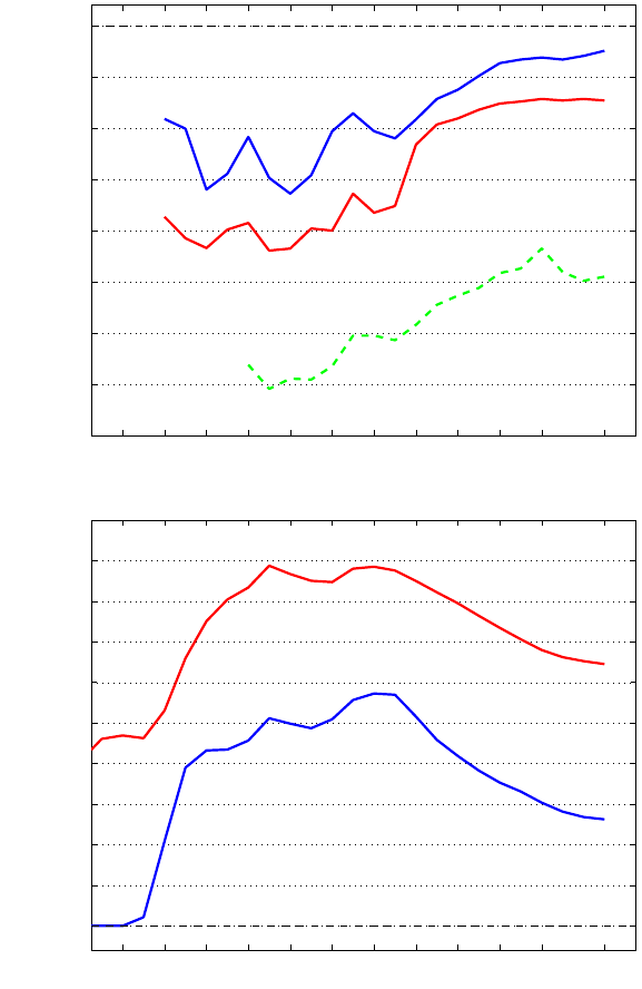
Average LTV

100

Loan-to-Value in %

48 50 52 54

62 64

VA&

-FHA

-S&L loans

FHA and VA Market Share

Market Share in %

46 48 50

58 60

-VA

-FHA+VA

Figure 5. FHA and VA Loan Programs in the Immediate Postwar Era. In response to changes

in government policies, mortgages with no downpayments were preva lent in the 1950s and 19 60s, decades

befo re the mortgage crisis began.

Source: LTVs from Herzog and Earley (1970) a nd Market shares from series Dc948 (FHA), DC9 49 (VA) and

Dc934 (Total) fr om Carter et al. (2006).

% of Purchases

96 98

02 04 06 08

-LTV≥100

LTV≥95&

LTV>90&

-LTV>80

Figure 6. Distribution of Combined Loan-to-Value (LTV) Ratios on Home Purchases in

Massachusetts: 1990-2011. The top line shows that a majority of home buyers in Massachusetts put

down less than 20 percent in most years after 1990. These statistics include all mortgages taken out at the

time of purchase and encompass c ash buyers.

Source: Wa rren Group collection of data from Massachusetts deed registries and autho rs’ calculations.

The Growing Role o f Mortg age Companies Evolution of S&Ls

1970 1975 1980 1985 1990 1995

Percent

Market share of

mortgage

companies

Mortgage Company

Net acquisitions/

Total market&

100

150

200

1970 1975 1980 1985 1990 1995

in Billions of Dollars

S&L

Originations&

← S&L Sales

S&L Purchase%

Decline of the “Originate-to-Hold” Model

100

1970 1975 1980 1985 1990 1995

in Percent

Share of Net

Acquisitions by

Originators

→

Figure 7. Mortgage Statistics for Mortgage Companies and Savings and Loans: 1970-1997. The upper left panel shows that the market

share of mortgage companies, a type of mortgage bank that originates mortgages for sale to outside investors, began to grow rapidly in the late 1970s.

The upper right panel shows that after 1980, S&Ls sold most of the mortgages they orig inated, becoming much like mortgag e companies. The bottom

panel shows that the decline of the “originate-to-hold” model started long before the recent housing boom.

Source: Carter et al. (200 6).

Reference Portfolio

As of February 26, 2007. Goldman Sachs neither represents nor provides any assurances that the actual Reference Portfolio on the Closing Date or any future date will

have the same characteristics as represented above. See the final Offering Circular for the Initial Reference Portfolio.

Reference Obligations are designated as “Midprime” herein if the weighted average FICO score of the underlying collateral that secures such Reference Obligation is greater than

625. All other Reference Obligations are designated as “Subprime” herein.

Security Type

Notional

Amount CUSIP Fitch Moody's S&P Base WAL (yrs) Dated Date Legal Final Servicer

ABFC 2006-OPT1 M8 Subprime 22,222,222 00075QAM4 BBB Baa2 BBB 3.9 8/10/2006 9/25/2036 OOMC

ABFC 2006-OPT2 M8 Subprime 22,222,222 00075XAP2 BBB Baa2 BBB 4.1 10/12/2006 10/25/2036 OOMC

ABSHE 2006-HE3 M7 Subprime 22,222,222 04541GXK3 BBB Baa2 BBB 3.8 4/17/2006 3/25/2036 OOMC

ABSHE 2006-HE4 M7 Subprime 22,222,222 04544GAP4 BBB Baa2 BBB 3.8 4/28/2006 5/25/2036 SPS

ACE 2006-FM2 M8 Midprime 22,222,222 00442CAN9 Baa2 BBB 4.5 10/30/2006 8/25/2036 WFB

ACE 2006-OP2 M9 Subprime 22,222,222 00441YAP7 Baa2 BBB- 4.3 10/30/2006 8/25/2036 WFB

ARSI 2006-W1 M8 Subprime 22,222,222 040104RQ6 BBB+ Baa2 BBB+ 3.8 2/7/2006 3/25/2036 AQMC

CARR 2006-FRE1 M9 Subprime 22,222,222 144538AN5 BBB+ Baa2 A 3.8 6/28/2006 7/25/2036 FREM

CARR 2006-FRE2 M8 Subprime 22,222,222 14454AAN9 Baa2 BBB+ 4.2 10/18/2006 10/25/2036 FREM

CARR 2006-NC1 M8 Midprime 22,222,222 144531FF2 BBB Baa2 BBB+ 3.6 2/8/2006 1/25/2036 NCMC

CARR 2006-NC2 M8 Subprime 22,222,222 14453FAM1 BBB Baa2 BBB 3.8 6/21/2006 6/25/2036 CARR

CARR 2006-NC3 M9 Subprime 22,222,222 144528AN6 BBB- Baa2 BBB- 4.0 8/10/2006 8/25/2036 NCMC

CARR 2006-OPT1 M8 Subprime 22,222,222 144531FV7 BBB+ Baa2 A- 3.6 3/14/2006 2/25/2036 OOMC

CMLTI 2006-AMC1 M8 Subprime 22,222,222 17309PAL0 Baa2 BBB 4.1 9/28/2006 9/25/2036 AQMC

CMLTI 2006-NC1 M8 Subprime 22,222,222 172983AN8 Baa2 BBB 3.8 6/29/2006 8/25/2036 WFB

CMLTI 2006-WFH2 M9 Subprime 22,222,222 17309MAN3 Baa2 BBB- 4.0 8/30/2006 8/25/2036 WFB

CMLTI 2006-WMC1 M8 Midprime 22,222,222 17307G2F4 A- Baa2 BBB+ 3.7 1/31/2006 12/25/2035 WFB

CMLTI 2007-WFH1 M9 Subprime 22,222,222 17311CAM3 Baa2 BBB- 4.5 2/9/2007 1/25/2037 WFB

CWL 2006-24 M8 Subprime 22,222,222 23243HAN1 Baa2 BBB 4.9 12/29/2006 5/25/2037 CHLS

FFML 2006-FF11 M8 Midprime 22,222,222 32028PAP0 BBB Baa2 BBB 3.9 9/6/2006 8/25/2036 WFB

FFML 2006-FF12 M8 Midprime 22,222,222 32027GAN6 BBB Baa2 BBB 4.2 8/25/2006 9/25/2036 ALS

FFML 2006-FF14 M8 Midprime 22,222,222 32027LAP0 BBB Baa2 BBB 4.2 9/25/2006 10/25/2036 AURA

FFML 2006-FF15 M8 Midprime 22,222,222 32028GAP0 BBB Baa2 BBB 4.3 10/25/2006 11/25/2036 AURA

FFML 2006-FF16 M8 Midprime 22,222,222 320275AN0 Baa2 BBB+ 4.3 11/30/2006 12/25/2036 NCHL

FFML 2006-FF17 M8 Midprime 22,222,222 32028KAP1 BBB Baa2 BBB 4.4 11/25/2006 12/25/2036 ALS

FFML 2006-FF7 M8 Midprime 22,222,222 320277AP1 BBB Baa2 BBB 3.6 5/31/2006 5/25/2036 WFB

FFML 2006-FF9 M8 Midprime 22,222,222 320276AP3 BBB+ Baa2 BBB+ 3.7 7/7/2006 6/25/2036 WFB

FHLT 2006-A M7 Subprime 22,222,222 35729RAN6 BBB+ Baa2 BBB 3.9 5/10/2006 5/25/2036 WFB

FHLT 2006-B M8 Midprime 22,222,222 35729QAN8 BBB+ Baa2 BBB 4.4 8/3/2006 8/25/2036 WFB

FMIC 2006-2 M8 Midprime 22,222,222 31659EAM0 Baa2 BBB+ 4.1 7/6/2006 7/25/2036 WFB

FMIC 2006-3 M8 Midprime 22,222,222 316599AN9 Baa2 BBB 4.4 10/27/2006 11/25/2036 WFB

GSAMP 2006-FM2 M8 Midprime 22,222,222 36245DAN0 Baa2 BBB+ 4.0 9/29/2006 9/25/2036 WFB

HEAT 2006-3 M8 Midprime 22,222,222 437084UZ7 BBB+ Baa2 BBB+ 3.5 3/30/2006 7/25/2036 SPS

HEAT 2006-5 M8 Midprime 22,222,222 437096AQ3 BBB+ Baa2 BBB+ 3.8 6/25/2006 10/25/2036 WFB

HEAT 2006-6 M8 Midprime 22,222,222 437097AP3 A- Baa2 A- 4.0 8/1/2006 11/25/2036 SPS

HEAT 2006-7 M8 Midprime 22,222,222 43709NAP8 BBB+ Baa2 BBB+ 4.2 10/3/2006 1/25/2037 SPS

HEAT 2006-8 M8 Midprime 22,222,222 43709QAP1 BBB Baa2 BBB+ 4.4 12/1/2006 3/25/2037 SPS

IXIS 2006-HE3 B2 Midprime 22,222,222 46602UAM0 BBB Baa2 BBB 4.8 9/29/2006 1/25/2037 WFB

JPMAC 2006-CW2 MV8 Midprime 22,222,222 46629BBA6 BBB Baa2 BBB 4.3 8/8/2006 8/25/2036 CWHL

JPMAC 2006-FRE1 M8 Midprime 22,222,222 46626LFV7 BBB Baa2 BBB 3.6 1/27/2006 5/25/2035 JPM

JPMAC 2006-WMC3 M8 Midprime 22,222,222 46629KAP4 BBB Baa2 BBB 4.3 9/14/2006 8/25/2036 JPM

LBMLT 2006-11 M8 Midprime 22,222,222 542512AN8 Baa2 BBB 4.7 12/14/2006 12/25/2036 WMB

LBMLT 2006-4 M8 Midprime 22,222,222 54251MAN4 Baa2 A- 3.9 5/9/2006 5/25/2036 WMB

LBMLT 2006-6 M8 Midprime 22,222,222 54251RAN3 BBB+ Baa2 BBB+ 4.2 7/26/2006 7/25/2036 WMB

LBMLT 2006-7 M8 Midprime 22,222,222 54251TAN9 BBB+ Baa2 A- 4.2 8/30/2006 8/25/2036 WMB

Reference Portfolio

Security Type

Notional

Amount CUSIP Fitch Moody's S&P Base WAL (yrs) Dated Date Legal Final Servicer

LBMLT 2006-WL1 M8 Midprime 22,222,222 542514RD8 Baa2 BBB 3.1 2/8/2006 1/25/2036 LBMC

MABS 2006-HE5 M9 Subprime 22,222,222 576455AN9 Baa2 BBB- 4.5 12/28/2006 11/25/2036 WFB

MABS 2006-NC2 M9 Subprime 22,222,222 55275BAP2 BBB Baa2 BBB- 4.2 9/28/2006 8/25/2036 WFB

MABS 2006-WMC4 M8 Midprime 22,222,222 57645MAP7 Baa2 BBB+ 4.6 11/30/2006 10/25/2036 WFB

MLMI 2006-WMC1 B2A Midprime 22,222,222 59020U4H5 Baa2 BBB+ 3.6 2/14/2006 1/25/2037 WCC

MSAC 2006-HE7 B2 Subprime 22,222,222 61750MAP0 Baa2 BBB 4.9 10/31/2006 9/25/2036 CWHL

MSAC 2006-HE8 B2 Midprime 22,222,222 61750SAP7 Baa2 BBB 5.1 11/29/2006 10/25/2036 WFB

MSAC 2006-NC4 B2 Subprime 22,222,222 61748LAN2 BBB Baa2 BBB 4.5 6/23/2006 6/25/2036 WFB

MSAC 2006-NC5 B3 Midprime 22,222,222 61749BAQ6 Baa2 BBB- 5.3 11/28/2006 10/25/2036 CWHL

MSAC 2006-WMC1 B2 Midprime 22,222,222 61744CXV3 BBB+ Baa2 A- 4.2 1/26/2006 12/25/2035 JPM

MSAC 2006-WMC2 B2 Midprime 22,222,222 61749KAP8 BBB Baa2 BBB 4.7 6/28/2006 7/25/2036 WFB

MSAC 2007-NC1 B2 Subprime 22,222,222 617505AN2 Baa2 BBB 5.3 1/26/2007 11/25/2036 CWHL

MSC 2006-HE2 B2 Midprime 22,222,222 617451FD6 BBB Baa2 BBB+ 4.5 4/28/2006 3/25/2036 WFB

MSIX 2006-2 B2 Midprime 22,222,222 617463AM6 Baa2 BBB 5.0 11/28/2006 11/25/2036 SAX

NHEL 2006-5 M8 Subprime 22,222,222 66988YAN2 Baa2 BBB+ 4.0 9/28/2006 11/25/2036 NOVA

NHELI 2006-FM1 M8 Midprime 22,222,222 65536HCF3 Baa2 BBB+ 3.3 1/30/2006 11/25/2035 WFB

NHELI 2006-FM2 M8 Midprime 22,222,222 65537FAN1 BBB+ Baa2 BBB+ 4.1 10/31/2006 7/25/2036 WFB

NHELI 2006-HE3 M8 Subprime 22,222,222 65536QAN8 BBB+ Baa2 BBB+ 4.0 8/31/2006 7/25/2036 WFB

OOMLT 2007-1 M8 Subprime 22,222,222 68400DAP9 Baa2 BBB 4.3 1/24/2007 1/25/2037 OOMC

SABR 2006-FR1 B2 Midprime 22,222,222 81375WJY3 BBB+ Baa2 A- 4.6 2/23/2006 11/25/2035 HSC

SABR 2006-FR3 B2 Subprime 22,222,222 813765AH7 BBB+ Baa2 BBB 5.0 8/3/2006 5/25/2036 HSC

SABR 2006-HE2 B2 Subprime 22,222,222 81377AAM4 BBB+ Baa2 BBB 4.1 9/28/2006 7/25/2036 HSC

SAIL 2006-4 M7 Subprime 22,222,222 86360WAM4 BBB Baa2 BBB 4.1 6/25/2006 7/25/2036 ALS

SASC 2006-EQ1A M8 Subprime 22,222,222 86360RAN3 Baa2 BBB 5.2 7/17/2006 7/25/2036 AURA

SASC 2006-OPT1 M7 Subprime 22,222,222 86359UAN9 BBB Baa2 BBB 3.7 4/25/2006 4/25/2036 AURA

SURF 2007-BC1 B2 Subprime 22,222,222 84752BAQ2 Baa2 BBB 4.9 1/24/2007 1/25/2038 WCC

SVHE 2006-EQ2 M8 Midprime 22,222,222 83611XAM6 BBB Baa2 BBB 4.6 12/28/2006 1/25/2037 OLS

SVHE 2006-OPT1 M7 Subprime 22,222,222 83611MMF2 BBB+ Baa2 BBB 3.6 3/10/2006 3/25/2036 OOMC

SVHE 2006-OPT2 M7 Subprime 22,222,222 83611MMT2 Baa2 A- 3.6 4/7/2006 5/25/2036 OOMC

SVHE 2006-OPT3 M7 Subprime 22,222,222 83611MPR3 Baa2 BBB 3.7 5/12/2006 6/25/2036 OOMC

SVHE 2006-OPT5 M8 Subprime 22,222,222 83612CAN9 Baa2 BBB 4.2 6/19/2006 7/25/2036 OOMC

ABSHE 2006-HE7 M9 Subprime 22,222,222 04544QAP2 BBB- Baa2 BBB- 4.4 11/30/2006 11/25/2036 SPS

BSABS 2006-HE9 M9 Subprime 22,222,222 07389MAP2 Baa2 BBB- 4.4 11/30/2006 11/25/2036 EMC

CMLTI 2007-AMC1 M8 Subprime 22,222,222 17311BAL7 Baa2 BBB 4.6 3/9/2007 12/25/2036 CWHL

FFML 2007-FF1 B2 Midprime 22,222,222 32028TAN7 Baa2 BBB 4.8 1/26/2007 1/25/2038 HLS

HASC 2006-HE2 M8 Midprime 22,222,222 44328BAP3 BBB+ Baa2 BBB+ 4.3 12/5/2006 12/25/2036 CMB

HEAT 2007-1 M8 Midprime 22,222,222 43710LAN4 BBB Baa2 BBB+ 4.5 2/1/2007 5/25/2037 SPS

LBMLT 2006-8 M8 Midprime 22,222,222 54251UAN6 Baa2 A- 4.4 9/21/2006 9/25/2036 WMB

LBMLT 2006-9 M8 Midprime 22,222,222 54251WAN2 Baa2 BBB+ 4.4 10/12/2006 10/25/2036 WMB

MLMI 2006-HE6 B3 Subprime 22,222,222 59023XAN6 Baa2 BBB- 4.6 12/28/2006 11/25/2037 WCC

MLMI 2006-OPT1 B2 Subprime 22,222,222 59022VAN1 Baa2 BBB 3.9 9/26/2006 8/25/2037 OOMC

MSAC 2007-HE1 B2 Subprime 22,222,222 617526AP3 Baa2 BBB 5.2 1/26/2007 11/25/2036 SM

OOMLT 2006-3 M9 Subprime 22,222,222 68389BAM5 Baa2 BBB- 4.0 10/27/2006 2/25/2037 OOMC

SASC 2006-WF3 M9 Subprime 22,222,222 86361EAP6 BBB- Baa2 BBB- 4.3 9/25/2006 9/25/2036 ALS

SVHE 2006-OPT4 M7 Subprime 22,222,222 83611YAM4 Baa2 BBB+ 3.6 5/26/2006 6/25/2036 OOMC

As of February 26, 2007. Goldman Sachs neither represents nor provides any assurances that the actual Reference Portfolio on the Closing Date or any future date will

have the same characteristics as represented above. See the final Offering Circular for the Initial Reference Portfolio.

Reference Obligations are designated as “Midprime” herein if the weighted average FICO score of the underlying collateral that secures such Reference Obligation is greater than

625. All other Reference Obligations are designated as “Subprime” herein.

Figure 8. The Reference Portfolio of the Abacus Deal. These two tables present the bonds

included in the Goldman Sachs Abacus deal. They illustrate that p otential investors in this deal had all the

information they needed to model the underlying cash ﬂows on the mortgages involved.

2006 V intage MBSs 2006 V intage CDOs

Figure 12: Moody’s downgrades and impairments of 2006 vintage RMBS.

Figure 13: Moody’s downgrades and impairments of 2006 vintage cash flow and hybrid ABS CDOs.

2007 V intage MBSs 2007 V intage CDOs

Figure 12: Moody’s downgrades and impairments of 2006 vintage RMBS.

Figure 13: Moody’s downgrades and impairments of 2006 vintage cash flow and hybrid ABS CDOs.

Figure 9. Downgrades and Impairments Among Mortgage-Backed Securities (MBS) and Collateralized Debt Obligations

(CDOs). The two panels on the left show that among private-lab e l MBS, lower-rated tranches suﬀere d massive losses. However, while a larg e

fraction of AAA-rated tranches were downgraded, the vast majority of these tranches paid oﬀ, as few of them suﬀered actual impairments. The two

panels on the right show tha t the same is not true for CDOs. Because these bonds tended to be backed by the lower -rated tranches of private-la bel

MBS, both the AAA-rated and the lower-rated tranches of CDOs suﬀered signiﬁcant impairments.

Source: Tables 12, 13, 17 and 18 in Financial Crisis Inquiry Commission (2010).

PSfrag

Market Share in %

2000

2001 20 02

2003

2004 2005 2006 2007

-Alt-A

Subprime&Subprime&

Figure 10. GSE Investments in Subprime and Alt-A Residential MBS: 2000-2007. This graph

shows that the government-sponsored housing enterprises, Fannie Mae and Freddie Mac, were signiﬁcant

purchasers of highly rated tranches of subprime and Alt-A securities during the hous ing b oom. As a share of

the overall subprime market, GSE purchases rose sharply in 2007 (note the change in vertical scale between 40

and 80 percent). This increase in shar e came about even though the absolute amo unt of subprime securities

purchased by the GSEs declined in 2007; the overall subprime market contr acted much more in perc e ntage

terms than GSE purchases did.

Source: Thomas and Van Or der (2011).

Payment changes and default

2007 2008 2009 2010 All

FRM share 38% 48 % 62% 74% 59%

Prior to delinquency spell that led to for eclosure...

% of loans

with...

Reset 18% 20 % 18% 11% 17%

Payment increase 12% 17 % 11% 9% 12%

Payment reduction 0% 0% 4% 8% 4%

No change since orig. 88% 82% 85% 83% 84%

Private Label 68% 54 % 37% 23% 41%

# obs in thous. 374 641 874 756 2,646

Relative Performance of Subprime ARMs and FRMs

All Subprime Subprime FRMs Subprime 2/28s

# of orig.

in thou.

P (default)

# of orig.

in thou.

in %

P (default)

# of orig.

in thou.

in %

P (default)

2005 529 41.9 198 37.3 37.1 332 62.7 44.8

2006 504 55.9 258 51.2 50.7 246 48.8 61.4

2007 246 55.9 208 84.5 53.8 38 15.5 66.8

Total 1278 50.1 663 51.9 47.6 615 48.1 52.8

Table 1. Payment Changes and Defaults among Various Mortgage Types. The top table shows

that a small minority of borrowers who eventually lost their homes to foreclosure experienced a payment

increase be fore they ﬁrst became delinquent. Payment increases preceded initial delinquency for only 12

percent of borrowers. Eighty-four perc e nt of borrowers who eventually lost their homes were making the

same payment at the time of initial delinquency as when they ﬁrst took out their loans. The bottom table

shows that 52.8 percent of subprime borrowers with adjustable-rate 2/28 mortgages originated from 2005 to

2007 defaulted. The comparable percentage for ﬁxed-rate mortgages is 47.6 p e rcent—only a few per c e ntage

points lower.

Source: authors’ calculations using data from Lender Processing Ser vices, Inc.

Name Scenario Probability Cum Loss

(1) Aggressive 11% HPA over the life of the p ool 15% 1.4%

(2) 8% HPA for life 15% 3.2%

(3) Base HPA slows t o 5 % by end-2005 50% 5.6%

(4) Pessimistic 0% HPA for the next 3 years 5% thereafter 15% 11.1%

(5) Meltdown -5% for the next 3 years, 5% thereafter 5% 17.1%

Table 2. Conditional Forecasts of Losses on Subprime Investments from Lehman Brothers.

This ta ble shows tha t investor s knew that subprime investments would turn sour if housing prices fell. The

“meltdown” s c e nario fo r housing prices above implies cumulative losses of 17.1 percent on subprime-backed

bonds; s uch losses would be large enough to wipe out all but the highest-rated tranches of most subprime

deals. The table also shows that investors placed small probabilities on these adverse price scenar ios, a fact

that explains why they were so willing to buy these bonds.

Source: “HEL Bond Proﬁle Across HPA Scenarios” from Lehman Brothers: “U.S. ABS Weekly Outlook,”

August 15, 2005 .

Date of Data from Title

12/8/06 10/06 “More widespread declines with early stabilization signs”

1/10/07 11/06 “Continuing declines with stronger stabilization signs”

2/6/07 12/06 “Tentative stabilization in HPA”

3/12/07 1/07 “Continued stabilization in HPA”

9/20/07 7/07 “Near bottom on HPA”

11/2/07 9/07 “UGLY! Double digit declines in August and September”

Table 3. Views on House Price Appreciation from JPMorgan Analysts. Even as housing prices

began to fall from their elevated levels, many analysts believed tha t prices would soon stabilize. The table

provides further evidence tha t investors were optimistic about house prices during the boom.

Source: Flanagan e t al. (2006b).

Institution Loss Institution Loss

($ billions) ($ billions)

1 Citigroup 42.9 11 Washington Mutual 9.1

2 UBS 38.2 12 Credit Agricole 8.3

3 Merrill Lynch 37.1 13 Lehman Brothers 8.2

4 HSBC 19.5 14 Deutsche Bank 7.6

5 IKB Deutsche 15.9 15 Wachovia 7.0

6 Royal Bank of Scotland 15.2 16 HBOS 7.0

7 Bank of America 15.1 17 Bayerische Landesbank 6.7

8 Morgan Stanley 14.1 18 Fortis 6.6

9 JPMorgan Chase 9.8 19 Canadian Imperial (CIBC) 6.5

10 Credit Suisse 9.6 20 Barclays 6.3

Table 4. Mortgage-Related Losses to Financial Institutions from the Subprime Crisis, as

of June 18, 2008. The date is cho sen prior to the Lehman bankrupcty to avoid contaminatio n from wider

ﬁnancial crisis. This table shows that mortgage industry insiders were the biggest losers fro m the housing

crash, despite the claims of the inside job theory of the crisis.

Source: Bloomberg (http://www.bloomberg.com/apps/news?pid=newsarchive&sid=a5GaivCMZu_M).

Entity Loans HELOC Ag ency Non-Ag ency CDOs Residential Total

+2nds MBS AAAs (r esi. subs) subs

Exposure

US banks/Thrifts 2,020 869 852 383 90 0 4,212

GSEs/FHLB 444 0 741 308 0 0

1,493

Broker/Dealers 0 0 49 100 130 24 303

REITs 0 0 82 10 0 0 92

Hedge Funds 0 0 50 51 0 24

126

Money Managers 0 0 494 225 0 24 743

Insurance Cos. 0 0 856 125 65 24 1,070

Overseas 0 0 689 413 45 24 1,172

Financial Guarant ors 0 62 0 0 100 0 162

Others 461 185 550 21 45 0 1,262

Total 2,925 1,116 4,362 1,63 6 476 121 10,680

Table 5. Exposure of Financial Institutions to Housing Risk on the Eve of the Crisis. This table shows that despite their ostensible use

of the originate-to-dis tribute model, investment banks retained large amounts of subprime ris k on their balance sheets. In particular, broker/dealers

held $130 billion in collateralized debt obligations (CDOs) that were ultimately backed by residential mortgages. These investments would suﬀer

massive losses when the subprime bonds backing them defaulted en masse during the ﬁnancial crisis.

Source: Figure 4 fr om “Residential Credit Losses—Going into Extra Innings?” Lehman Brothers U.S. Securitized Products, April 11, 2008 a nd

reprinted in Acharya and Richardson (2009).