
DOCUMENT RESUME
ED 389 710
TM 024 190
AUTHOR
Stocking, Martha L.
TITLE
Scale Drift in On-Line Calibration.
INSTITUTION
Educational Testing Service, Princeton, N.J.
SPONS AGENCY
Office of Naval Ref.earch, Arlington, VA. Cognitive
and Neural Sciences Div.
REPORT NO
ETS-RR-88-28-0NR
PUB DATE
May 88
CONTRACT
N0001.4-83-K-0457
NOTE
l50p.
PUB TYPE
Reports
Evaluative/Feasibility (142)
EDRS PRICE
MFOI/PC06 Plus Postage'.
DESCRIPTORS
*Adaptive Testing; *Computer Assisted Testing; Item
Banks; *Item Response Theory; *Online Systems;
Psychometrics; Simulation; *Test Items
IDENTIFIERS
Armed Services Vocational Aptitude Battery;
*Calibration; LOGIST Computer Program; *Scale
Drift
ABSTRACT
Recent advances in psychometrics and computer
technology encourage the development of model-based methods of
individualized testing on a microcomputer, where each examinee
receives short tests and where the number of pretest items that can
be administered is severely restricted. On-line (i.e., data is
collected on operational equipment) methods for calibrating pretest
items in this setting face new challenges. In the context of adaptive
testing (CAT) ,
two LOCIST-based methods of on-line calibration that
were developed are described. These two methods were applied and
compared in a simulation study using data from the CAT Armed Services
Vocational Aptitude Battery. One of the methods was superior to the
other in terms of statistical properties, but the superior method was
more expensive to implement in terms of the numbers of items required
and either the numbers of examinees or numbers of items per examinee
required. Both methods showed scale drift, although the drift was in
opposite directions for the two methods. Ways to reduce scale drift
are explored. An appendix contains 4 tables and 22 figures, and 17
references are attached. (Author/SLD)
***********************************************************************
*
Reproductions supplied by EDRS are the best that can be made
*
from the original document.
***********************************************************************

U S DEPARTMENT Of EDUCATION
Office
ducafional Research and improvement
E DU .ATIONAL RE SOURCES INFORMATION
CENTER rERICI
Etus document has been reproduced as
ece.ve0 Rom the Person w orpanrzabon
or Kj.nafing 1
f ' Mmor changes nave beer made to Improve
rePrOductOn Quaid,
P0,nts 01 y.e 0r 0dImans Slated .n Ih.s 00C u
cnen1 00 1101 nee
,.SsarrIy
epresenl ourc.al
OE RI 00S.fion Or POI.CT
SCALE DRIFT IN ON-LINE CALIBRATION
Martha L. Stocking
RR-88-28-0NR
This research was sponsored in part by the
Cognitive Science Program
Cognitive and Neural Sciences Division
Office of Naval Research, under
Contract No. N00014-83-K-0457
Contract Authority Identification No
NR 150-520
Frederic M. Lord, Principal Investigator
Educational Testing Service
Princeton, New Jersey
May 1988
Reproduction in whole or in part is permitted
for any purpose of the United States Government.
Approved for public release: distribution unlimited.
BEST COPY AVAILABLE
Ave

Unclassified
SECURITY CLASSIFICATION 0,- THIS PAGE
REPORT DOCUMENTATION PAGE
Form Approved
OMB No 0704-0188
la REPORT SECURITY CLASSiFICATION
Unclassified
lb RESTRICTIVE MARKINGS
2a SECURITY CLASSIFICATION AUTHORITY
3
DISTRBuTION /AVAILABILITY OF REPORT
Approved for public release;
distribution unlimited.
2b DECLASSIFICATION/DOWNGRADING SCHEDULE
4 PERFORMING ORGANIZATION REPORT NUMBER(S)
RR-88-28-0NR
5 MON'TORING ORGANIZATION REPORT NUMBER(S)
6a. NAME OF PERFORMING ORGANIZATION
Educational Testing Service
6b OFFICE SYMBOL
licae(If app
)
bl
1
7a NAME OF MONITORING
ORGANIZATIOTognitive Scienc
Program, Office of Naval Research
(1142PT), 800 Tiprrh Quincy
Srrper
6c ADDRESS (City, State, and ZIP Code)
Princeton, NJ
08541
7b ADDRESS (City, State, and ZIP code)
Arlington, VA
22217-5000
8a. NAME OF FUNDING:SPONSORING
ORGANIZATION
8b. OFFICE SYMBOL
(If applicable)
9 PROCuREMENT INSTRUMENT IDENTIFICATION NUMBER
N00014-83-K-0457
8c. ADDRESS (City, State. and ZIP code)
10 SOURCE OF FUNDING NUMBERS
PROGRAM
ELEMENT NO
61153N
PROJECT
NO
RR04204
TASK
NO
RR04204-01NR
WORK UNIT
ACCESSION NO
150-520
11
TITLE (Include Security Classification)
Scale Drift in On-Line Calibration (Unclassified)
12 PERSONAL AUTHOR(S)
.
Martha L. Stocking
13a TYPE OF REPORT
Technical
TIME COVERED
FROM
TO
14 DATE OF REPORT (Year,Month, Day)
May 1988
15 PAGE COUNT
122
16 SUPPLEMENTARY NOTATION
17
COSATI CODES
18 SUBJECT TERMS (Continue on reverse if necessary and identify by block number)
Adaptive testing
1RT scales
Item pools
Calibration
FIELD GROUP
SUB-GROUP
05
10
19 ABSTRACT (Continue on reverse if necessary and identify by block number)
Recent advances in psychometrics and computer technology encourage
the
development of model-based methods of individualized testing on a
microcomputer, where each examinee receives short tests and the
number of
pretest items that can be administered is severely
restricted.
On-line (i.e.,
data is collected on operational equipment) methods for
calibrating pretest
items in this setting face new challenges.
In the context of adaptive testing,
two LOGIST-based methods of on-line cal"Jration were
developed and are
described.
These two methods are tried out and compared in a simulation
study
using data for the CAT-ASVAB.
20 DISTRIBUTION/AVAILABILIIY
or ABSTRACT
El uNCLASSIPIED/uNunwED 0 SAME AS RP1
El DTIC UM PS
21 ABSTRACT SECURITY CL ASSIFICATION
Unclassified
22a NAME OF RESPONSIB_E INDIVIDUAL
Dr. Imes Lester
22b TELEPHONE (Include Area Code)
202-696-4503
22c OFFICE SYMBOL
ONR 1142C5
DD Form 1473, JUN 86
Previous editions are obsolete
S/N 0102-LF-014-6603
St CURITY CI ASSIFICATION OF THIS PAGE
Unclassified

Scale Drift
1
Scale Drift in On-Line Calibration
Martha L. Stocking
Educational Testing Service
Princeton, New Jersey
May 1988
,i

Copyright 01988.
Educational Testing Service.
All rights reserved.

Scale Drift
2
Abstract
Recent advances in psychometrics and computer technology
encourage the development of model-based methods
of individualized
testing on a microcomputer, where each examinee receives short
tests and the number of pretest items that can be administered
is
severely restricted.
On-line (i.e., data is collected on
operational equipment) methods for calibrating pretest items in
this setting face new challenges.
In the context of adaptive
testing, two LOGIST-based methods of on-line calibration were
developed and are described.
These two methods are tried out and
compared in a simulation study using data for the CAT-ASVAB.
Keywords:
Adaptive testing
Item pools
IRT scales
Calibration

Scale Drift
3
Introduction
Conventional modes of testing, where every examinee takes a
single test form (or parallel versions of it) in large
administrations using paper and pencil as the delivery and
recording medium, belong to the past.
Recent advances in both
psychometrics and computer technology seem to point in the
direction of model-based methods of individualized testing on a
microcomputer, where each examinee receives short tests and
testing is generally done on a demand basis.
Much has been
written about adaptive testing in this latter context.
But other
new methods of testing, for example model-based mastery testing or
work-sample testing, may also be designed as short tests
administered by computer to small samples of examinees.
Traditional methods of estimating parameters for items,
particularly model-based parameters as opposed to conventional
psychometric parameters such as proportions-correct, depend upon
relatively large numbers of examinees taking relatively large
numbers of items.
This is especially true for the more frequently
used complex models, such as the 3-parameter logistic model.
Model-based testing requires, moreover, item parameter estimates
in order to design tests.
The challenge is to develop new methods
of item parameter estimation (calibration) that capitalize on
Scale Drift
4
computerized testing modes without destroying the advantages of
short computerized tests.
These methods are generally referred to
as 'on-line' calibration methods because the data collected for
calibration of new items comes from the administration of these
items on operational equipment as part of an examinee's testing
session.
In some contexts, the acquisition of sufficient numbers of
examinees for adequate parameter estimation in on-line calibration
may be problematical.
In these situations, it may be possible to
accumulate a reasonable number of examinees over a realistic time
frame.
If this is not feasible, then on-line calibration methods
that are more optimal for this situation than those described here
need to be developed.
Even if the number of examinees is sufficient, a central
problem, in any application of on-line calibration, is how to
obtain adequate calibrations of pretest items when both the length
of the computerized test is very short and the number of extra
items that can be administered in pretest mode to an examinee is
severely restricted.
The current context of the particular
methods of on-line calibration reported here is adaptive testing
for the Armed Services Vocational Aptitude Battery (ASVAB).
The
results, however, are more general and apply to other modes of

Scale Drift
5
computerized testing that rely on recent advances in psychometric
theory.
Remaining sections of this paper will describe the current
project and its design, two methods of on-line calibration based
on the estimation procedures in the LO(.,IST computer program
(Wingersky, 1983) and the efficacy of these methods in the context
of adaptive testing, and how these and othcr similar on-line
calibration methods might be improved in the context of adaptive
testing as well as other types of computerized testing.
The Current Project
A number of agencies of the Department of Defense funded a
three-year project to develop and evaluate different methods of
on-line calibration for the computerized adaptive Armed Services
Vocational Aptitude Battery (CAT-ASVAB).
Although exploration of
general classes of item calibration methods was encouraged in this
context, final results were constrained to be parameterized as the
3-parameter logistic model of item response functions.
The final
phase of this project consisted of a series of 'high-fidelity'
simulations of adaptive testing and item pool refreshment.
The
simulations are called 'high-fidelity' for two reasons.
First,
the true item response functions and ability densities, both
developed by Levine (1987) are nonparametric, and therefore more

Scale Drift
6
realistic than more restrictive parametric models.
Second, the
study design represents a realistic scenario for on-line
calibrations for the adaptive ASVAB as well as many other types of
computerized tests.
Two LOGIST-based methods of on-line
calibration were investigated.
As part of the same project,
Darrell Bock (1987), Michael Levine (1987), and Fumiko Samejima
(1987) investigated other methods of on-line calibration.
The results presented here provide some general guidance for
effective computerized test item pool construction and
maintenance.
In addition, one LOGIST-based method is superior to
the other in terms of statistical properties.
However, the
superior method is more expensive to implement in terms of the
numbers of items required, and either the numbers of examinees
required or the numbers of items per examinee.
The Study DeSign
Figure 1 displays the overall design of the study.
Although
four experimenters participated, only the details of the LOGIST-
based methods indicated on the right side of Figure 1 will be
discussed in detail below.
Using data provided by Vale
(Prestwood, Vale, Massey and Welsh, 1985), nonparametric item
response functions and ability densities were produced by Levine
(1987) to serve as true item response functions and ability

Scale Drift
7
densities.
Also using Vale's data, LOGIST was run to provide
parameter estimates for subsequent use.
Items were selected for
an initial pool and calibrated by each experimenter.
Then four
rounds adaptive test simulations and item pool refreshment were
conducted.
The Original Data (Block 1 of Figure 1)
Vale, et al., developed over 2000 experimental items to be
considered as candidates for the original ASVAB adaptive testing
item pool.
A subset of these items, developed for the Word
Knowledge (WK) subtest, was used in this study.
The WK subtest
consists of a single item type, synonyms, and is designed to
measure the understanding of words typically used in
social
studies and everyday life, human relationships, science and
nature, and arts and humanities (Prestwood, et al., 1985).
The
focus of the Vale item development effort was to write and
calibrate similar items that spanned a wider range of difficulty
than those found in operational use.
Vale developed a total of 258 such WK items.
For the purpose
of obtaining item parameter estimates he obtained a sample of
N
8171 candidates for military service from Military Entrance
Processing Stations who had also taken the conventional ASVAB test
battery.
This set of data, that is, the responses of 8171

Scale Drift
8
individuals to the 'experimental' Word Knowledge items as well as
the conventional ASVAB, forms the basis of the current study.
A calibration of the experimental WK items using the computer
program LOGIST was performed.
This calibration is noted in the
top block in Figure 1.
Table 1 shows summary statistics for the
item parameter estimates obtained from LOGIST.
The items were
designed to be different from a conventional test aimed at the
average examinee; the purpose was to obtain items for an adaptive
test item pool.
The items are supposed to be very discriminating,
with low guessing parameters, and span a wide range of difficulty.
As seen in Table 1, the items are indeed more discriminating than
is customarily seen.
Although the items span a wide range of
difficulty, there are more easier items relative to the number of
harder items.
Insert Figure 1 and Table 1 about here
Summary statistics for the ability estimates of the
calibration sample are also shown in Table 1.
Although this
sample of people was the only one available for the purpose of
calibrating these experimental items, the sample may not be
completely appropriate.
Examinees were informed that their scores
Scale Drift
9
on the experimental item did not count.
It is therefore possible
that the motivation of individuals was not the same as motivation
presumably will be in the intended population.
The Definition of Truth (Block 1 of Figure 1)
Using the data provided by Vale, Levine produced
nonparametrin item response functions and ability densities to be
used as true item response functions and ability densities in this
study.
Figure 2 shows the true item response functions for some
typical items.
In general, these true item response functions are
nonmonotonic.
Insert Figure 2 about here
In Vale's data collection design, no examinee was
administered all 258 experimental items.
Rather, the items were
broken up into three blocks of 86 items that were roughly parallel
to each other.
Each block was administered to a subset of
examinees.
Therefore Levine produced three nonparametric ability
densities.
To produce a description of a single ability density,
Davis (1987) averaged the three densities, and then interpolated,
integrated, and normalized the resulting function.
All simulated
examinees (simulees) are drawn from the resulting distribution.

Scale Drift
10
Initial Item Selection (Block 2 of Figure 1)
An initial set of 100 items was drawn by Davis from the 258
experimental items to form the first adaptive test item pool.
Research has shown (Hulin, Drasgow and Parsons, 1983) that item
pools much larger than this are not necessary for short adaptive
tests.
To select the 100 items, Davis used the LOGIST parameter
estimates summarized in Table 1 to compute a table of items sorted
by their estimated information functions at various levels of
ability.
Items yielding successively decreasing amounts of
information were selected until 100 unique items were obtained.
There were two constraints on the process used by Davis.
First, 10 items that were judged to be excessively non-3PL in
shape on the basis of observed data were eliminated from the 258
before selection was done.
These non-3PL items exhibited either
severe nonmonotonicities or broad plateaus in the mid-range of
ability.
Second, the ability metric was divided into intervals of
1.0 between -3.0 and +3.0, and the numbers of items selected from
each of the two most extreme intervals was constrained to be no
more that 10, while 20 items were selected from each of the
remaining intervals.
This latter constraint was to control for
the fact that there are proportionally too many easy items in
Vale's original item set.

Scale Drift
11
The Simulated Initial Calibration (Block 2 of Figure 1)
Up to this point in the study design, Vale's WK data have
been used to develop a definition of truth for the simulations,
and to provide estimated parameters for the purpose of selecting
the initial 100 item pool.
But these parameter estimates are no
longer appropriate for subsequent steps.
They represent 3PL
estimates of the true item response functions that are
hypothesized to underlie the responses collected by Vale from live
examinees.
These item response functions are not the same as
those generated by Levine to be used as the (non-3PL) definition
of truth for this study.
Instead, it is necessary to obtain 3PL
parameter estimates from data where Levine's true item response
functions generate responses to items from simulees.
This step is
a simulated initial calibration of the 100 item pool.
Davis divided the 100 items into four 25-item subsets, each
of which had approximately the same estimated test information
function based on LOGIST parameter estimates.
Each of N
6000
simulees was administered two subsets of 25 items in an
overlapping design that provided 3000 simulee responses per item.
Responses to the items were generated using the true (non-3PL)
item response functions and simulee abilities.
LOGIST was run on
these data to provide estimated item parameters for the 100 items

Scale Drift
12
in the Round 0 adaptive test item pool.
These parameters
estimates were then returned to Davis for the next step in the
simulation study.
A Typical Round in the Simulation Study (Blocks 3 through 6,
Figure 1)
A typical Round in the simulation study consisted of the
simulation of an adaptive test (by Davis), the selection and
seeding of candidate new items for the adaptive test item pool (by
Davis), the identification of items to be removed (by Davis), and
the calibration and selection of new items to be included in the
next Round of simulations (by individual experimenters).
Davis
performed his functions separately by experimenter, and, for the
results reported here, separately by the two LOGIST-based methods
of on-line calibration.
Thus the items in the pool, the item
parameter estimates, and adaptive test simulations may differ for
each experimental method at each Round.
This process was repeated
for a total of four Rounds.
For each Round, Davis simulated the administration of a 15-
item fixed-length adaptive test to a sample of N
15,000 simulees
drawn at random from the composite ability density.
The same
sample of simulees was used for each experimental method within a
Round.
Owen's (1975) Bayesian procedure was used to update

Scale Drift
13
ability estimates during the adaptive test.
The next item to be
administered during the test was chosen to be that item that was
most informative at the estimated ability, except for the
imposition of efforts to control item exposure. 'Exposure'
parameters controlled the probabilities with which an optimally-
selected item was actually administered to a simulee.
For the
first item, this probability was .2, for the second item the
probability was .25, for the third it was .33, for the fourth it
was .5, and for the fifth through the fifteenth, this probability
was 1.0.
Item usage data was collected by Davis for each item, and
accumulated across each Round in the simulations.
At each Round,
the 25 most used items of the current 100 item pool were
identified as items that must be replaced for the next Round.
In
addition, for each Round, Davis identified a pool of candidate
'new' items by randomly selecting 50 items from the full set of
Vale's original 258 items.
Within a Round, the same 50-item set
of candidate new items was used for each experimental Method.
Response data were collected for these items by administering each
simulee 5 randomly selected items from this set of 50. On
average, each new item had about 1500 responses to be used in the
subsequent estimation of item parameters by each experimenter.

Scale Drift
14
Responses to these new items played no role in item selection or
ability estimation during the course of the adaptive test.
The Final 'Half' Round (Block 7 of Figure 1)
At the end of four Rounds, the original 100-item pool has
been 'refreshed' four times.
In order to examine the cumulative
effects of these four Rounds on simulee ability, Davis conducted a
final half-Round, consisting of just the simulation of an adaptive
test using this final item pool.
Two LOGIST-based Methods of On-line Calibration
A Note on Methods That Do NOT Work
Lord (1984) described a straightforward approach to on-line
calibration that did not work.
Since the logic underlying this
approach is so appealing, it is instructive to examine it.
The
basic idea of this approach was to simultaneously calibrate the
candidate new items and recalibrate the entire adaptive test item
pool.
Since the results of such a calibration would not be on the
same scale as the original item pool, it would be necessary to
determine a transformation of these results to that scale.
Using
the relationship between the item parameter reestimates for the
adaptive test pool and the original item parameter estimates for
these same items, a suitable scaling transformation could be
determined by minimizing the difference between the test

Scale Drift
15
characteristic curves for the two different sets of estimates, as
in Stocking and Lord (1983).
After such a transformation had been
applied, the calibration results for the candidate new items would
also be on the scale of the adaptive test item pool.
This basic
plan of simultaneous calibration of candidate new items and the
current adaptive test item pool, along with a transformation,
would then be repeated for each Round of the simulation study.
A problem with this approach is that some of the items in the
adaptive test item pool may not have been administered frequently
enough to provide adequate data for subsequent recalibration.
To
solve this problem, those items that were infrequently used in the
adaptive test were administered nonadaptively to a sufficient
number of examinees for adequate calibration.
Thus, in Lord's
design, there were three types of items to be calibrated,
distinguishable by the nature of the data available for
calibration purposes.
The first type consisted of candidate new
items for which only nonadaptive responses were collected.
The
second type consisted of items already in the pool, but whose
response rate was sufficiently low in the adaptive test that some
nonadaptive administrations had been performed to increase the
number of responses per item.
The third type consisted of items
already in the pool, but whose response rate was sufficiently high

Scale Drift
16
that only adaptive test responses were required for adequate
calibration.
The third type of item, that is, those items for which only
adaptive responses were obtained, causes severe problems when
attempting to estimate parameters for the 3PL.
Since their
response rate is high in the adaptive test, these are the more
discriminating items in the pool. The more discriminating an
item, the greater the change in the probability of a correct
answer for small changes in ability close to the item difficulty.
Since the adaptive test works well, these items are usually
administered to simulees with very similar levels of ability.
Thus the distribution of ability for those simulees administered
this kind of item becomes more concentrated the better the
adaptive test works. These highly discriminating items divide
this concentrated ability distribution into two classes:
those
simulees whose ability lies slightly below the item difficulty and
therefore have only a small probability of responding correctly,
and those simulees whose ability lies slightly above the item
difficulty and therefore have a high probability of responding
correctly.
The observed data from which item parameters are to be
estimated are the actual item responses from the simulees.
These
data also tend to be divided into two classes by the highly
Scale Drift
17
discriminating item -- those who respond correctly and those who
respond incorrectly.
These responses are not sufficient to
estimate item discrimination or the lower asymptote.
This
situation is illustrated for a few items in Figure 3 (taken from
Lord, 1984), where the boxes represent observed proportions
correct for particular ability groups and are plotted proportional
in size to the number of cases in the group.
In the extreme case,
for an infinitely long adaptive test in which the estimated
ability becomes indistinguishable from the true ability, the
response data from which three item parameters must be estimated
collapses into a single point located at the item difficulty, with
the observed proportion of correct responses halfway between
chance and 1.0.
Insert Figure 3 about here
Calibration procedures such as LOGIST, that do not utilize
other information that might be available about the item
parameters, cannot perform adequately on items such as these for
which only adaptive responses are available.
Mislevy (personal
communication, 1987) conjectures that any other currently
available estimation procedure would encounter similar

Scale Drift
18
difficulties in trying to estimate 2PL or 3PL parameters from
these adaptive responses, unless these adaptive responses were
augmented by additional information, such as prior distributions
on item parameters or responses from examinees over a broader
range of ability.
The solution is not to discard the items in this set from the
calibration and simply proceed with the two remaining sets of
items. This is equivalent to discarding the better (more
discriminating) items available and using only the poorer (less
discriminating) items in the pool as a scale anchor. Instead it
appears that one solution could lie in the direction of avoiding
the direct use of adaptive test responses by summarizing the
information available from the adaptive test when estimating
parameters for the new items. Both methods described below move
in this direction.
Method A
For this method, adaptive test item responses and parameter
estimates for items already in the adaptive test item pool are
used to compute a maximum likelihood estimate of simulee ability.
This estimated ability serves as a summary of information
available from the adaptive test.
A LOGIST calibration run is
then performed in which these ability estimates are fixed, and
Scale Drift
19
nonadaptive responses to the new seeded items are used to estimate
parameters for the 50 candidate new items.
The top half of Figure
4 shows the details of this method across all four Rounds,
starting with Round 1.
Insert Figure 4 about here
Because the ability estimates are fixed in the calibration of
the new items, and no rescaling is done within the LOGIST run, the
ability estimates determine the scale on which the item parameter
estimates are reported.
Since the ability estimates themselves
are on the scale of the adaptive test item pool, the estimates for
the candidate new items will be also.
Method B
This method requires a set of 'anchor' items to be seeded,
along with the new items.
The purpose of the anchor items is to
try to improve upon Method A.
Method A depends entirely upon
treating estimates of ability as if they were, in fact, true
abilities in order to maintain the scales of subsequent item
pools.
In so doing, errors will be made because estimated
abilities differ from true abilities.
The anchor items will be
used to attempt to correct for scale drift that may result from

Scale Drift
20
the use of these imperfect ability estimates for scale
maintenance.
It seems reasonable to select as anchors items that are
representative of those in the adaptive test item pool in terms of
difficulty.
This is because scale transformations that are
.derived from the anchor items will be applied to all items to be
considered as candidates for item pools.
In addition, the quality
of the anchor items, in terms of item information, should be no
worse than typical items produced for the adaptive test item pool,
since it makes no sense to develop scale transformations based on
items of poor quality.
For purposes of this study, 25 anchor items were defined to
be exactly like 25 items selected from the original 100-item pool.
The first step in the selection process was to eliminate from
further consideration 9 items of the 100-item pool that were
judged to be poorly fit by the 3PL in Round 0.
The remaining 91
items were grouped on the basis of estimated difficulty into 5
equal intervals between -2.0 and 2.0.
Five items were then
selected randomly from each interval to be the anchor items.
Nonadaptive responses to 5 randomly selected new items and 5
randomly selected anchor items were collected from each simulee.
Since there are half as many anchor items as there are new items.

Scale Drift
21
each new item received about 1500 responses and each anchor item
received about 3000 responses.
The alternative design in which
each simulee received only 5 seeded items, either new or anchor
items, requires more simulees before an on-line calibration can
occur, and was judged inconvenient to implement for the purposes
of this study.
Thus, the doubling of response rate for anchor
items is not a requirement of this Method, but an artifact of the
chosen design.
As in Method A, adaptive test information is summarized in a
maximum likelihood estimate of simulee ability.
A LOGIST
calibration is done, fixing the ability estimates and estimating
item parameters for the 50 new items and the 25 anchor items.
Using the reestimates for the anchor items, and their initial
estimates from Round 0, a scaling transformation is chosen to
minimize the difference between the two test characteristic curves
(Stocking & Lord, 1983).
Using this tranformation the results of
this LOGIST run are placed on the scale of the Round 0 item pool.
The bottom half of Figure 4 shows the details of
Method B across
all four Rounds, beginning with Round 1.
The Selection of New Items
Although the calibration of new items at each Round differed
for the two Methods studied, the same algorithm was used to select

Scale Drift
22
from the 50 candidate items the 25 new items to be included in the
next Round's item pool.
The difference between the estimated test
information function for the Round 0 item pool and the estimated
test information function for the 75 items to remain from the
current pool was defined as a 'target' information function.
The
use of this difference as a target insures that items will be
selected to maximize the resemblance of the next Round's item pool
to the Round 0 item pool.
Three methods of selecting item sets or 'drafts' to match the
target information function were tried.
The first method selected
items to minimize the maximum difference between the target and
the draft test information functions across the ability metric
from -3.0 to +3.0.
The second method selected items with the
greatest area under their item information functions within
ability levels that appeared important based on the target
information function.
A third method was a combination of these
two:
a draft set of 25 items was selected on the basis of the
area under the item information functions and then attempts were
made to improve on this draft by discarding some items and
selecting others that minimized the maximum difference between the
target and the draft test information functions.
Scale Drift
23
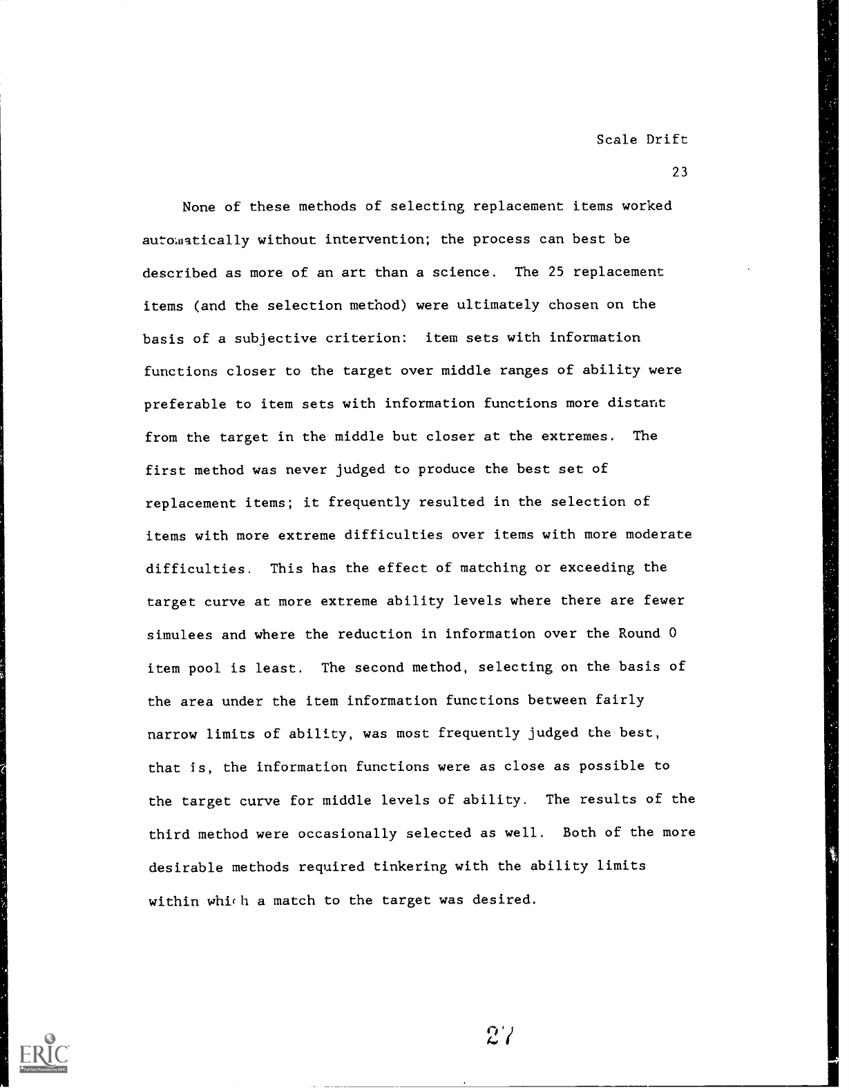
None of these methods of selecting replacement items worked
autowatically without intervention; the process can best be
described as more of an art than a science.
The 25 replacement
items (and the selection method) were ultimately chosen on the
basis of a subjective criterion:
item sets with information
functions closer to the target over middle ranges of ability were
preferable to item sets with information functions more distant
from the target in the middle but closer at the extremes.
The
first method was never judged to produce the best set of
replacement items; it frequently resulted in the selection of
items with more extreme difficulties over items with more moderate
difficulties.
This has the effect of matching or exceeding the
target curve at more extreme ability levels where there are fewer
simulees and where the reduction in information over the Round 0
item pool is least.
The second method, selecting on the basis of
the area under the item information functions between fairly
narrow limits of ability, was most frequently judged the best,
that is, the information functions were as close as possible to
the target curve for middle levels of ability.
The results of the
third method were occasionally selected as well.
Both of the more
desirable methods required tinkering with the ability limits
within whiih a match to the target was desired.

Scale Drift
24
Results, Part 1:
The True Score Metric
In examining the results of on-line calibration by any
Method, it seems important to first focus attention on global
effects in a metric that approximates one in which examinee scores
will be reported.
A subsequent section will examine in more
detail the operation of each Method in the IRT metric.
The number-right true score metric for the Round 0 pool was
chosen for this series of comparisons because the Round 0 pool is
the only item pool that is constant across Methods, and, indeed,
across all other experimenters in this project.
In this context,
the items in the Round 0 pool may be viewed as a "reference" test
that is common to all experimenters.
A true score on this common
reference test is the score a simulee woul,t have obtained if
administered the entire Round 0 pool as a conventional test.
The conditional RMSE between estimated number-right true
score and true score, and the conditional bias in
estimated
number-right true score were computed for each Method after each
Round.
True scores were computed using true simulee abilities for
a Round and the true IRF's for the Round
0 items.
Estimated
number-right true scores were computed using simulee abilities
estimated from the adaptive test at each Round, and the estimated
IRF's for the Round 0 items.
For small intervals of true score,
Scale Drift
25
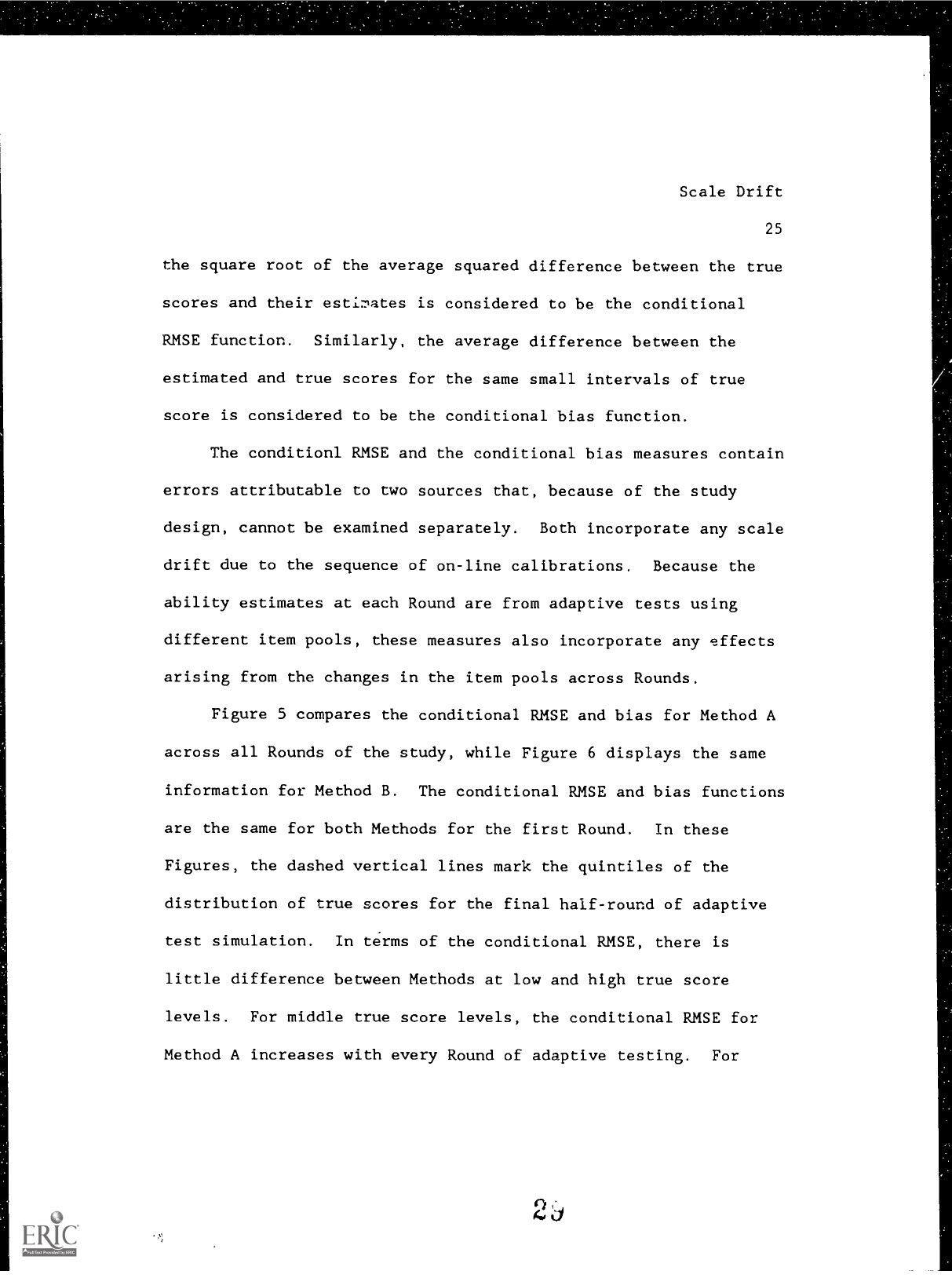
the square root of the average squared difference between the true
scores and their estizlates is considered to be the conditional
RMSE function.
Similarly, the average difference between the
estimated and true scores for the same small intervals of true
score is considered to be the conditional bias function.
The conditionl RMSE and the conditional bias measures contain
errors attributable to two sources that, because of the study
design, cannot be examined separately.
Both incorporate any scale
drift due to the sequence of on-line calibrations.
Because the
ability estimates at each Round are from adaptive tests using
different item pools, these measures also incorporate any effects
arising from the changes in the item pools across Rounds.
Figure 5 compares the conditional RMSE and bias for Method A
across all Rounds of the study, while Figure 6 displays the same
information for Method B.
The conditional RMSE and bias functions
are the same for both Methods for the first Round.
In these
Figures, the dashed vertical lines mark the quintiles of the
distribution of true scores for the final half-round of adaptive
test simulation.
In terms of the conditional RMSE, there is
little difference between Methods at low and high true score
levels.
For middle true score levels, the conditional RMSE for
Method A increases with every Round of adaptive testing.
For

Scale Drift
26
these same true score levels, the Method B RMSE tends to remain
about the same after an initial increase from the first to the
second Round of adaptive testing.
For middle true score levels,
where most of the simulees are located, Method B generally has a
smaller RMSE than Method A.
Insert Figures 5 and 6 about here
The changes in the conditional bias functions appear to be
systematic, although in different ways, across Rounds for both
Methods.
For Method A, the bias becomes more positive across
Rounds for true scores slightly above the median and more negative
for low true scores.
For Method B the eirection of the bias is
opposite for middle true scores -- higher levels show more
negative bias and lower levels show more positive bias across
Rounds.
Method B tends to have smaller absolute bias than Method
A across all Rounds.
Figure 7 displays the conditional RMSE and bias for both
methods after the end of all Rounds of adaptive test simulations.
This Figure clarifies the
and high true scores, the
true scores, Method B has
comparisons of the two Methods.
For low
RMSE functions are similar; at middle
smaller RMSE.
For the very lowest and
Scale Drift
27
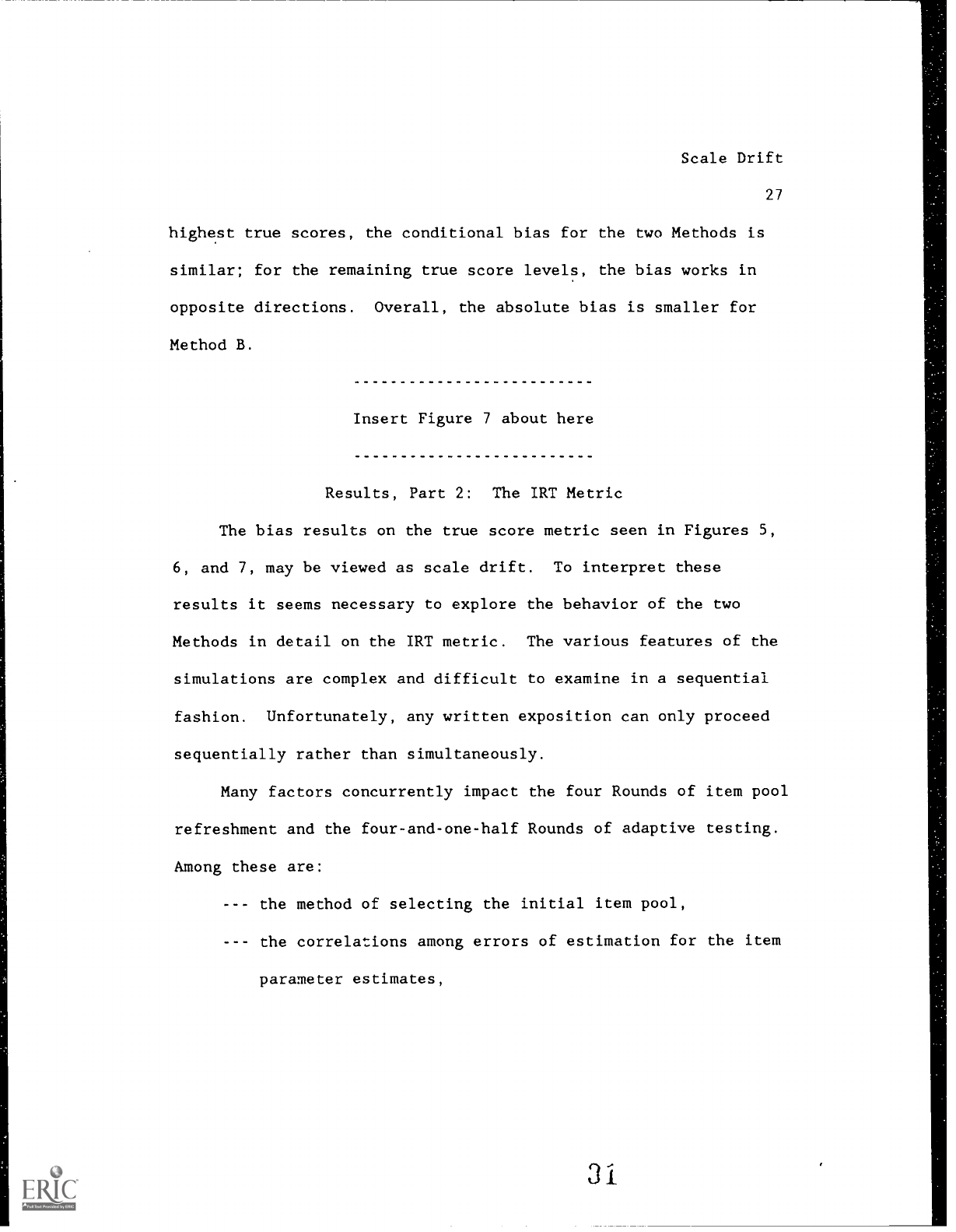
highest true scores, the conditional bias for the two Methods is
similar; for the remaining true score levels, the bias works in
opposite directions. Overall, the absolute bias is smaller for
Method B.
Insert Figure 7 about here
Results, Part 2: The IRT Metric
The bias results on the true score metric seen in Figures 5,
6, and 7, may be viewed as scale drift.
To interpret these
results it seems necessary to explore the behavior of the two
Methods in detail on the IRT metric.
The various features of the
simulations are complex and difficult to examine in a sequential
fashion.
Unfortunately, any written exposition can only proceed
sequentially rather than simultaneously.
Many factors concurrently impact the four Rounds of item pool
refreshment and the four-and-one-half Rounds of adaptive testing.
Among these are:
--- the method of selecting the initial item pool,
--- the correlations among errors of estimation for the item
parameter estimates,

Scale Drift
28
--- the adaptive testing paradigm that selects items for
administration based on an estimated ability and
estimated item information,
--- the use of ability estimates in place of true abilities,
--- the precision with which new items are calibrated,
--- the method of identifying items in the current pool for
replacement,
--- the method of selecting replacement items from the new
items.
The effort to ,,nderstand the interactions among these factors
is complicated by other factors that are not central to on-line
calibration, but must be dealt with nevertheless.
Among these
complicating factors are:
--- the necessity of establishing a single IRT scale upon
which comparisons can be made,
--- the comparison of estimated parametric IRF's with true
nonparametric counterparts,
--- the fact that changes in relevant variables between
consecutive Rounds may be small, necessitating the
examination of multiple Rounds simultaneously and across
two different Methods.

Scale Drift
29
The information available from each Method for each Round
will be described in five different but overlapping analyses.
The
first such analysis deals with what, for lack of a better term,
may be called a 'snapshot' of a single Round.
Included in this
snapshot are data about I) the item pool at the beginning of the
Round, 2) the nature of the ability estimates obtained from using
this item pool to administer adaptive tests, 3) the nature of the
errors made when using these ability estimates as if they were
true abilities, and 4) the estimation of the parameters for the
candidate new items.
The remaining analyses will look at many of these same
features summarized in different ways.
Given an item pool, the
second analysis will explore what happens to ability estimation
when this pool is used to administer adaptive tests.
This
analysis will take place across Rounds within Methods of on-line
calibration.
The third analysis will investigate what happens to
the calibration of candidate new items, given that the ability
estimates are used as if they are true abilities.
This analysis
will also take place across Rounds within Methods.
The foulth
analysis will focus in detail on the differences in the
calibration of new items between Methods across Rounds, with
particular attention paid to considering separately the effects of

Scale Drift
30
the approximate scaling transformation for Method B. Finally,
given the rules for elimination of items and the method of
selecting new items for the adaptive test pool, the fifth analysis
will explore the impact of these across Rounds and within Methods.
The Establishment of a Single IRT Metric
Throughout these discussions, comparisons of estimated
quantities are made with their true counterparts.
This, of
course, is one of the advantages of a simulation study.
Before
this comparison can be made, however, true and estimated
quantities must be on the same (arbitrary) metric.
It is unlikely that the metric on which the true item
response functions and abilities were developed by Levine bears
any simple linear relationship with the metric of LOGIST
estimates.
However, the assumption is made here that a linear
transformation can be developed that will be a good approximation
to a possibly more complex transformation.
From the simulated
initial calibration of the Round 0 item pool we have abilities
estimated by LOGIST.
Davis provided the corresponding true
abilities for the N = 6000 simulees.
Robust measures of location
and scale (Mosteller & Tukey, 1977, p.20) were computed for both
the estimated and true abilities and a linear transformation
developed from them to transform true abilities to the scale of

Scale Drift
31
the Round 0 calibration.
This same transformation was applied to
the true abilities of all other simulees in the remaining Rounds
of the study.
All true item response functions were transformed to the
Round 0 scale by applying this approximate linear transformation
to Levine's tabled ability values.
Figure 8 shows the transformed
true item response functions (solid lines) and the LOGIST
estimates of the same item response functions (dotted lines) on
the Round 0 metric for some typical items.
All subsequent
comparisons with true values were done using the transformed true
item response functions and abilities.
Insert Figure 8 about here
Some Results From the Bivariate Normal Distribution
Some aspects of the subsequent discussions, particularly
those dealing with true and estimated abilities, may at first
appear confusing.
This section attempts to deal in advance with
these aspects by removing them temporarily from the context of on-
line calibration, and placing them in the more familiar context of
the bivariate normal distribution.
The point of the exercise is
not to imply that the joint distribution of estimated and true

Scale Drift
32
abilities is bivariate normal, but rather to clarify some of the
techniques used in subsequent analyses.
Suppose we have two variables whose joint distribution is
bivariate normal
'
z
1
and z
2
. Suppose that both variables have
means of 0 and variances of 1, and that the correlation between
the two is rho < 1. A scatterplot of 400 random draws from such a
distribution, restricted to the range of -1 to +1, is shown in the
left panel of Figure 9. On the same panel, the solid line is the
45-degree line of 12 = zl. The line with long dashes is the
regression of
12 on z l'
namely z
2
= rho * z
1
. The line with the
short dashes is the regression of z
1
on Z
2'
Z
1
= rho * z
2'
or 12
(1/rho) * zl.
Insert Figure 9 about here
Consider the difference (z, - z1).
The expectation of this
residual, conditional on z
l'
is
E(z z11z1) = E(z21z1)
-
z1 rho * zi - 11 = (rho
1) * 11.
This function is plotted as a function of 11 in the middle panel
of Figure 9.
Because rho is less than 1, this function has a
negative slope.
Suppose that zi is an unobservable variable, and

Scale Drift
33
the z
2
is an observable estimate of it. The average value of this
residual for different values of the unobservable variable is, by
definition, a conditional bias function.
Consider the expectation of this same residual, now
conditional on z
2:
E(z2 z11z2) = z2 E(z11z2) = z2 rho * z2 = (1 rho) * z2.
This function is plotted as a function of z
2
in the right panel of
Figure 9.
Because rho is less than 1, this function has a
positive slope. We again suppose that z
1
is an unobservable
variable, and z
2
is an observable estimate of it. The average
value of this residual for different values of the observable
variable can be considered to be a conditional error function.
That is to say, it gives the average of the errors that will be
made if the observable variable is used as if it were the
unobservable variable, for different values of the observable
variable.
In subsequent sections, the joint distributions of estiwted
and true ability will be analyzed in both ways.
The expected
residuals conditional on the true abilities will constitute an
examination of the bias in the estimated abilities.
These
Scale Drift
34
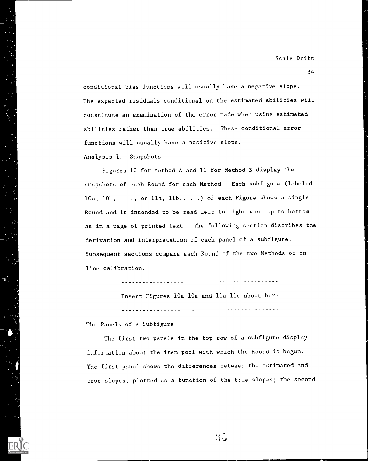
conditional bias functions will usually have a negative slope.
The expected residuals conditional on the estimated abilities will
constitute an examination of the error made when using estimated
abilities rather than true abilities.
These conditional error
functions will usually have a positive slope.
Analysis 1:
Snapshots
Figures 10 for Method A and 11 for Method B display the
snapshots of each Round for each Method.
Each subfigure (labeled
10a, 10b,.
.
, or lla, lib,.
.
.) of each Figure shows a single
Round and is intended to be read left to right and top to bottom
as in a page of printed text.
The following section discribes the
derivation and interpretation of each panel of a subfigure.
Subsequent sections compare each Round of the two Methods of on-
line calibration.
Insert Figures 10a-10e and lla-lle about here
The Panels of a Subfigure
The first two panels in the top row of a subfigure display
information about the item pool with which the Round is begun.
The first panel shows the differences between the estimated and
true slopes, plotted as a function of the true slopes;
the second

Scale Drift
35
panel shows the differences between the estimated and true
difficulties, plotted as a function of the true difficulties.
In
the second panel, the difficulty of an item for which the slope
has been overestimated is indicated by a plus, and the difficulty
of an item for which the slope has been underestimated is
indicated by a circle.
In these and all other figures containing item parameter
information, the 'true' difficulty is defined as that value on the
true (transformed) ability metric that yields the same probability
of a correct response as does the estimated difficulty on the
estimated item response function.
The 'true' slopes are computed
by numerical methods (Hamming, 1962, p. 318) at the location of
the true difficulty.
Thi-z method of obtaining 'true' difficulty
and slope parameters for the nonparametric true IRF's is flawed.
Consider an item represented by a particular true nonparametric
IRF.
If we have two different estimates of the difficulty
parameter for this item, it is possible that this procedure will
produce two different values of the 'true' difficulty parameter,
and also two different values of the 'true' slope parameter.
To
examine the magnitude of this problem, the 50 new items calibrated
in Round 4 were examined.
These items are the same for each
Method, and the difference between the parameter estimates, and

Scale Drift
36
therefore between the 'true' parameters determined by this Method,
should be largest on this final Round.
The average difference
between the 'true' difficulties was found to be .02, and the
average difference between the 'true' slopes was found to be .004.
These differences are small.
This method has an additional disadvantage.
In this and
subsequent figures, not all relevant items may appear.
The
nonparametric item response function is described by tabled
function values over a finite interval of ability, and
occasionally it is not possible to find the 'true' difficulty and
slope values within this table.
Appendix 1 contains a list, by
Figure, of all items that should, but do not, appear in plots of
this nature throughout this paper, along with the values of their
estimated item parameters.
In spite of these flaws, this method of determining 'true'
parameters from nonparametric item response functions, although
crude, seems to to work well enough to give useful insights into
differences between the two Methods of on-line calibration.
The third panel in the top row of each snapshot displays the
median difference between estimated and true ability as a function
of the median true ability for small intervals of true ability.
The median difference rather than the average difference is used
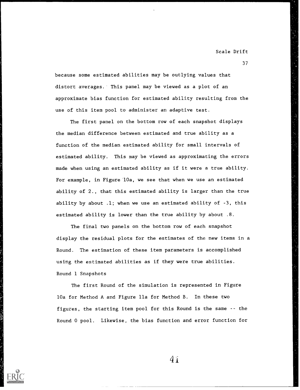
Scale Drift
37
because some estimated abilities may be outlying values that
distort averages.
This panel may be viewed as a plot of an
approximate bias function for estimated ability resulting from the
use of this item pool to administer an adaptive test.
The first panel on the bottom row of each snapshot displays
the median difference between estimated and true ability as a
function of the median estimated ability for small intervals of
estimated ability.
This may be viewed as approximating the errors
made when using an estimated ability as if it were a true ability.
For example, in Figure 10a, we see that when we use an estimated
ability of 2., that this estimated ability is larger than the true
ability by about .1; when we use an estimated ability of -3, this
estimated ability is lower than the true ability by about .8.
The final two panels on the bottom row of each snapshot
display the residual plots for the estimates of the new items in a
Round.
The estimation of these item parameters is accomplished
using the estimated abilities as if they were true abilities.
Round 1 Snapshots
The first Round of the simulation is represented in Figure
10a for Method A and Figure lla for Method B.
In these two
figures, the starting item pool for this Round is the same -- the
Round 0 pool.
Likewise, the bias function and error function for
Scale Drift
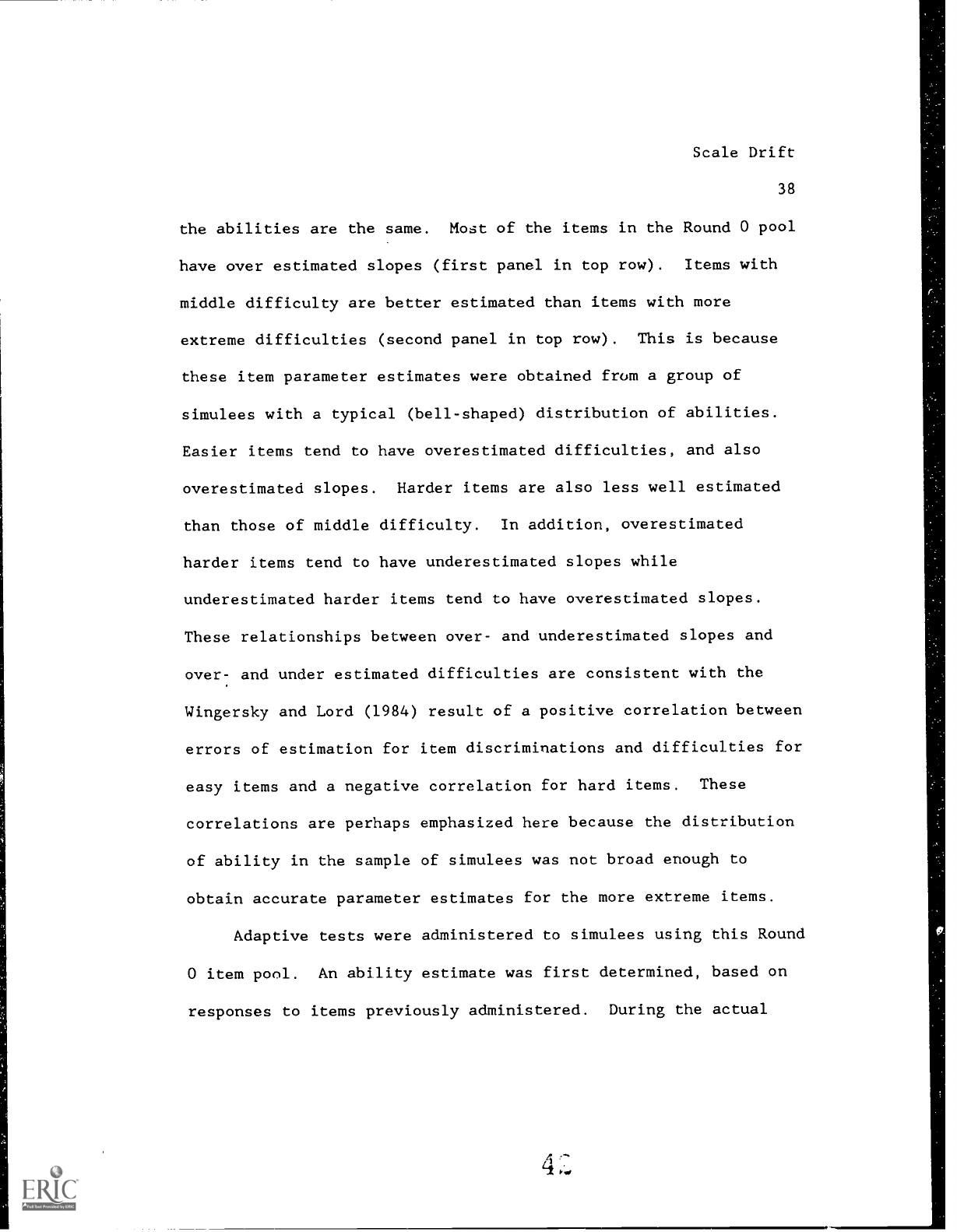
38
the abilities are the same.
Most of the items in the Round 0 pool
have over estimated slopes (first panel in top row).
Items with
middle difficulty are better estimated than items with more
extreme difficulties (second panel in top row).
This is because
these item parameter estimates were obtained from a group of
simulees with a typical (bell-shaped) distribution of abilities.
Easier items tend to have overestimated difficulties, and also
overestimated slopes.
Harder items are also less well estimated
than those of middle difficulty.
In addition, overestimated
harder items tend to have underestimated slopes while
underestimated harder items tend to have overestimated slopes.
These relationships between over- and underestimated slopes and
over: and under estimated difficulties are consistent with the
Wingersky and Lord (1984) result of a positive correlation between
errors of estimation for item discriminations and difficulties for
easy items and a negative correlation for hard items.
These
correlations are perhaps emphasized here because the distribution
of ability in the sample of simulees was not broad enough to
obtain accurate parameter estimates for the more extreme items.
Adaptive tests were administered to simulees using this Round
0 item pool.
An ability estimate was first determined, based on
responses to items previously administered.
During the actual

Scale Drift
39
operation of the adaptive test, this ability estimate was computed
using Bayesian methods developed by Owen (1975).
For both Methods
of on-line calibration, a maximum likelihood ability estimate,
rather than Owen's Bayesian ability estimate, was used.
Both the
Owen's Bayesian ability estimate and the maximum likelihood
ability estimate weight items with higher estimated
discriminations more than items with lower estimated
discriminations.
In the adaptive test, items that were maximally informative
at the estimated ability were then selected for administration.
The information for an item is itself an estimate, and will be an
overestimate of true information for items with overestimated
slopes.
For items of approximately the same difficulty, the items
with the most overestimated slopes will be chosen more frequently
than items with less overestimated slopes.
Because of the
correlation between errors of estimation for difficulty and
discrimination, easy items with overestimated difficulties will be
chosen more frequently than easy items with less overestimated
difficulties.
Likewise harder items with underestimated
difficulties will be chosen more frequently than harder items with
less underestimated difficulties. The missestimation of
difficulties will be emphasized by methods of estimating ability

Scale Drift
40
that weight items with higher estimated slopes more than items
with lower estimated slopes.
We can expect these speculations to be confirmed by the bias
plot of estimated abilities.
Indeed, the bias in the ability
estimates (third panel of top row in Figures 10a and 11a) does
follow the same pattern as that of the difficulties of the items
with overestimated slopes (middle panel of top row in Figures 10a
and 11a).
In the next step of Round 1 for both Methods, the ability
estimates are used as if they were true abilities and the item
parameters are estimated for the candidate new items.
We know
that estimated abilities have a larger variance that true
abilities.
Because the unit of measurement of the IRT scale is
usually taken to be the standard deviation of abilities, this
difference in variance may be viewed as a difference in scale.
Table 2 displays the variance of the true and estimated abilities
for all samples of simulees for all Rounds.
While the differences
in the Round 1 variances may seem quite small, a better picture of
the nature of the errors incurred is found in the error function
panel (first panel of bottom row in Figures 10a and 11a).
Higher
estimated abilities are systematically overestimates of their
corresponding true values, and the difference becomes larger as

Scale Drift
41
the estimated ability increases.
The same is true in the opposite
direction for lower estimated abilities.
Insert Table 2 about here
Up to this point in Round 1, the two Methods of on-line
calibration have been identical.
It is in the calibration of the
new items that the Methods begin to differ.
The spreading out of
the estimated abilities and their subsequent use as if they were
true abilities causes the slopes to be generally underestimated
for the new items for Method A (middle panel, bottom row, in
Figure 10a).
The difficulties for the new items are not as well
estimated as the difficulties for the Re 'nd 0 pool; the scatter of
the residuals is greater.
In addition the trend towards the
overestimation of difficulty for harder items and underestimation
of difficulty for easy items is consistent with the direction
predicted on the basis of correlation between estimation errors
for items with generally underestimated slopes.
The calibration of new items for Method B (second and third
panels, bottom row, Figure 11a) is less affected by the use of
estimated abilities as if they were true abilities.
About half of
the items have overestimated slopes.
The difficulties for the

Scale Drift
42
items with overestimated slopes are missestimated in a pattern
consistent with the correlation of estimation errors.
The
difficulties for the items with underestimated slopes seem less
affected.
The items are the same for both Methods and the
parameters are estimated from the same set of estimated abilities.
What is different is the scaling transformation that is performed
for Method B, using information from the anchor items.
This has
the effect of an approximate correction for the fact that using
the estimated abilities to obtain parameter estimates is not the
same as using true abilities. From this point on, the two Methods
of on-line calibration will differ, and the differences will
become more notable with each Round.
Round 2 Snapshots
Figure 10b for Method A and Figure llb for Method B display
the second Round of simulation results.
Items have been discarded
from the Round 0 pool on the basis of the frequncy of use in
adaptive test simulations.
Because the simulees are a typical
group, the most frequently used items were the discriminating
items of middle difficulty.
Replacements were selected from the
new items calibrated in the previous Round (Figures 10a and lla,
bottom row, third panel).
These items spanned a broad range of
difficulty.
All items of middle difficulty were selected as

Scale Drift
43
replacements, as well as more extreme items with higher estimated
slopes.
The Method A pool for Round 2 contains more items with
underestimated slopes than the Method B pool. .The well estimated
middle difficulty items from Round 0 have been eliminated for both
Methods, and replaced by items whose difficulties are less well
estimated.
For Method B, and also, but less clearly, for Method
A, the pattern of residuals for the item difficulties for items
with overestimated slopes is consistent with the correlation of
estimation errors; the trend is less clear for items with
underestimated slopes.
As in Round 0, the bias in the estimated
abilities follows the bias in item difficulties for those items
with overestimated slopes.
For both Methods, the variance of estimated abilities is
greater than the variance of true abilities, although this
difference is smaller than the differences for Round 1, as shown
in Table 2.
But, also for both Methods, the pattern of errors
made when using estimates as if they were true shows systematic
errors are now made, even for middle levels of estimated ability.
It seems probable that this phenomenon is the result of the fact
that the item difficulties are less well estimated for both

Scale Drift
44
Methods for middle difficulty items as well as the patterns of
missestimation of slopes and difficulties peculiar to a Method.
For Method A, estimated abilities just above the middle are
overestimates, while estimated abilities just below the middle are
underestimates. Method B shows the same error pattern for
estimated abilities just above the middle, and a slightly less
severe underestimation for estimated abilities just below the
middle.
For Method A, then, the estimated abilities are more
spread out than for Method B, even for middle ability estimates.
This difference in patterns is a consequence of the
underestimation of slopes for almost all new items selected for
inclusion in this Round 2 pool by Method A.
When using these estimated abilities to estimate parameters
for new items, as before the slopes for Method A are mostly
underestimated while those for Method B are less so.
The
correlation of estimation errors is now clearly visible for Method
A for those items with underestimated slopes.
It is also clearly
visible for Method B for those items with overestimated slopes.
Snapshots for Rounds 3, 4, and 5
The remaining subfigures of Figures 10 and 11 show the
results for the remaining Rounds.
All of the phenomena examined
so far appear and become more exaggerated as the Rounds progress:
Scale Drift
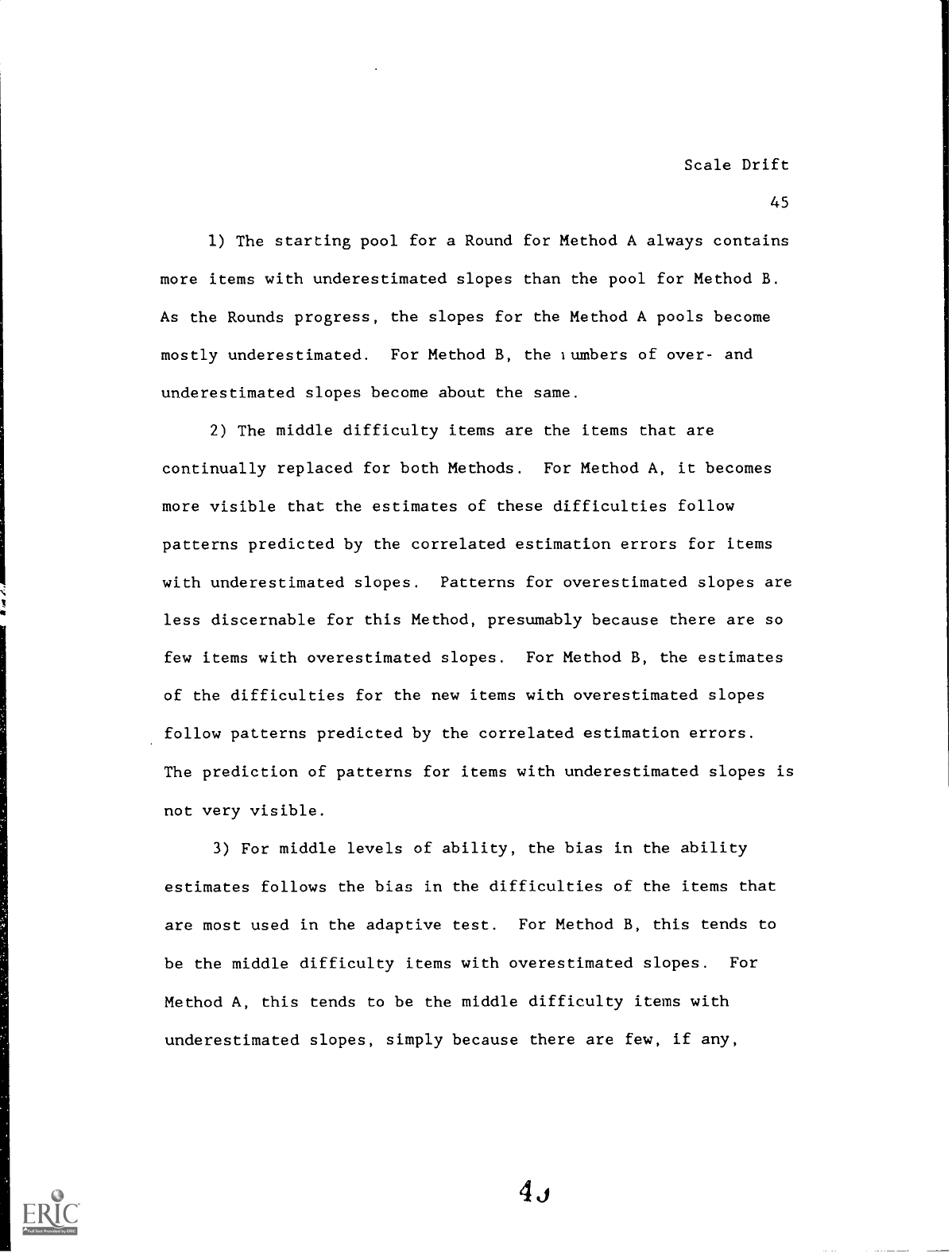
45
1) The starting pool for a Round for Method A always contains
more items with underestimated slopes than the pool for Method B.
As the Rounds progress, the slopes for the Method A pools become
mostly underestimated.
For Method B, the lumbers of over- and
underestimated slopes become about the same.
2) The middle difficulty items are the items that are
continually replaced for both Methods. For Method A, it becomes
more visible that the estimates of these difficulties follow
patterns predicted by the correlated estimation errors for items
with underestimated slopes.
Patterns for overestimated slopes are
less discernable for this Method, presumably because there are so
few items with overestimated slopes.
For Method B, the estimates
of the difficulties for the new items with overestimated slopes
follow patterns predicted by the correlated estimation errors.
The prediction of patterns for items with underestimated slopes is
not very visible.
3) For middle levels of ability, the bias in the ability
estimates follows the bias in the difficulties of the items that
are most used in the adaptive test.
For Method B, this tends to
be the middle difficulty items with overestimated slopes.
For
Method A, this tends to be the middle difficulty items with
underestimated slopes, simply because there are few, if any,

Scale Drift
46
Method A items calibrated on-line with overestimated slopes.
These biases tend to be in opposite directions, predictable on the
basis of the correlated estimation errors when the items were
calibrated on-line.
4) Table 2 shows that, across Rounds, the estimated abilities
are more spread out than the true abilities.
This difference is
generally larger for Method A than for Method B, and for Method A
it increases across Rounds.
The Figures show that for middle
levels of estimated ability, the errors made when using estimated
ability as if it were true become increasingly large in opposite
directions around the middle for Method A.
They remain about the
same for Method B.
This reflects fact that the slopes of items
for Method A are consistently underestimated, as well as the
missestimation of middle item difficulties for both Methods.
Analysis 2:
Item Pools and Bias in Ability Estimates
This analysis is offered as an aid in understanding a single
aspect of the data presented in the snapshots of
each Round.
Figure 12 for Method A and Figure 13 for Method B display for
each
Round the item pool with which the Round is begun, and the
approximate bias functions for the estimated abilities that result
when the item pool is used in adaptive testing.
These Figures are
constructed by lining up the top row of three panels from each

Scale Drift
47
subfigure in Figures 10 and 11.
Each row in the Figures 12 and 13
represents a Round in the simulation.
The top rows in the two
Figures are the same; they both display the Round 0 item pool and
the bias functions for the first Round of the simulation.
Although no new information is presented here, it may be easier to
comprehend the trends across Rounds when the panels are arranged
in this manner.
Insert Figures 12 and 13 about here
Looking down the left hand column in Figure 12, it is easy to
see that, for Method A, the point cloud representing the residuals
of the slopes is mostly above the horizontal line in Round 1,
gradually drifts downward, and is mostly below the horizontal line
in the final Round.
For Method B in Figure 13, this drift seems
to stabilize at about the point where the slopes are evenly over
and underestimated.
The middle column of panels in the two Figures shows that the
changes in the residuals of the difficulties are predominantly for
middle difficulty items.
These are the items that get used most
frequently, and therefore replaced most frequently.
For Method A,
these items become overestimated if they are slightly above the

Scale Drift
48
middle and underestimated if they are slightly below the middle.
Most of these items have underestimated slopes. For Method B,
these middle difficulty items have slopes that are both over- and
underestimated.
The third column of panels in the two Figures shows that the
bias in the estimated abilities tends to remain the same for
extreme abilities, regardless of the Method of on-line calibration
or the particular Round.
The bias of middle estimated abilities
changes because the middle difficulty items are being replaced.
For Method B, the bias tends to look like the bias in the
difficulties for items of middle difficulty that have
overestimated slopes.
This is because it is just those items that
are selected most frequently and weighted most heavily for
simulees of middle ability levels in adaptive testing.
For Method
A this bias also tends to look like the bias for items of middle
difficulty, because these are the only items available for
simulees of middle ability levels.
Most, if not all, of these
items have underestimated slopes.
Analysis 3:
Errors in Ability Estimates and the Calibration of
New Items
This analysis is offered as an aid to understanding a second
aspect of the data presented in the snapshots of each Round.
Scale Drift
49
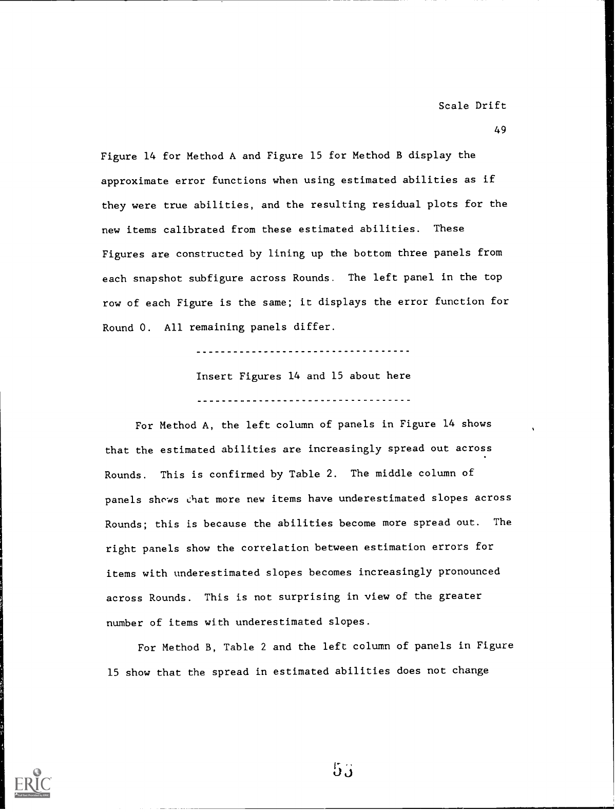
Figure 14 for Method A and Figure 15 for Method B display the
approximate error functions when using estimated abilities as if
they were true abilities, and the resulting residual plots for the
new items calibrated from these estimated abilities.
These
Figures are constructed by lining up the bottom three panels from
each snapshot subfigure across Rounds.
The left panel in the top
row of each Figure is the same; it displays the error function
for
Round 0.
All remaining panels differ.
Insert Figures 14 and 15 about here
For Method A, the left column of panels in Figure 14 shows
that the estimated abilities are increasingly spread out across
Rounds.
This is confirmed by Table 2.
The middle column of
panels shows chat more new items have underestimated slopes across
Rounds; this is because the abilities become more spread out.
The
right panels show the correlation between estimation errors for
items with underestimated slopes becomes increasingly pronounced
across Rounds.
This is not surprising in view of the greater
number of items with underestimated slopes.
For Method B, Table 2 and the left column of panels in Figure
15 show that the spread in estimated abilities does not change

Scale Drift
50
much across Rounds.
The middle column of panels shows that the
slopes for the new items are about evenly over- and
underestimated.
The right column of panels shows that correlation
betweell errors of estimation for items with overestimated slopes
becomes more visible across Rounds.
It is possible for individual item parameter estimates to be
different but the estimated item response functions produced by
these estimates to be similar.
This is particularly true for very
easy and very hard items, where individual item parameter
estimates are not well determined;
quite different parameter
estimates can give similar item response functions in the area of
the ability distribution where simulees are located.
It would be
instructive to compare estimated item response functions for both
Methods across Rounds.
Unfortunately, only a single item (Vale
number 244) was included in the Round 0 pool and was also included
in the 50 candidate new items for each Round for each Method.
This item was a discriminating item with higher than average
difficulty.
Figures 16 (Method A) and 17 (Method B) show the true
item response function (solid line) and the estimates of this item
response function across all Rounds.
Method A estimates show more
variability, both in terms of slope and location, than do Method B
estimates.
Method A estimated slopes tend to be too low and

Scale Drift
51
estimated difficulties too high.
Method B estimated slopes tend
to be too high and estimated difficulties too low.
Insert Figures 16 and 17 about here
While it is not possible to directly compare the estimated
item response functions for any other item across Rounds and
Methods, it is possible to approach issues of the accuracy of
estimation more indirectly.
Using the true abilities at a Round
as weights, a weighted RMSE between the estimated and true item
response functions was computed.
At each Round, an average
weighted RMSE was then computed, where the average was taken over
the new items calibrated in that Round.
Table 3 shows these
average weighted RMSE's for all Rounds for both Methods.
The
Round 0 average weighted RMSE is the same for both Methods since
the items and estimates of item parameters are identical.
The
average weighted RMSE for Method A increases across subsequent
Rounds, while the average RMSE for Method B remains approximately
the same.
Insert Table 3 about here

Scale Drift
52
Analysis 4:
The Calibration of New Items and the Approximate
Scaling Transformation
The Round 0 item pool is, by design, identical for both
Methods of on-line calibration.
After the first Round the actual
items included in a pool can be different for the two Methods,
also by design.
The differences are introduced by the elimination
of overused items and the selection of the 25 new items to be
included in the next item pool, processes that operated
independently for the two Methods.
In actuality, all items of the
100 in the final pool created for Round 1 were the same, 96 out of
100 were the same for Round 2, 95 were the same for Round 3, and
90 were the same for Round 4.
Since the pools are so similar for
the two Methods, the differences between the two Methods appear to
originate with the approximate scaling transformation developed
from the anchor items for Method B.
This analysis will examine
the effects of this rescaling in more detail.
The multiplicative and additive constants of each rescaling
are shown in Table 4.
All multiplicative constants are less then
one, indicating that at each Round, the scale unit before
transformation is too large.
All additive constants are non-zero,
indicating that the scale origin before transformation is not
precisely correct.
The importance to attach to the differences

Scale Drift
53
among the multiplicative constants or the differences among the
additive constants is unknown but could be investigated through a
jackknife study.
Insert Table 4 about here
Note that the rescalings depend upon one another in a complex
and indirect fashion.
The rescaling for Round 1 is applied to the
new items calibrated in that Round, of which 25 are selected to be
included in the second item pool.
To the extent that abilities in
the second Round of adaptive testing are estimated using the items
that have been calibrated on-line in Round 1, the calibration of
the new items in the second Round will be affected by the
rescaling from the first Round.
Since the 25 items selected are
of middle difficulty, it is certain that some abilities are
estimated from some items that have been calibrated on-line.
This
same type of dependency propagates across Rounds.
Figure 18 shows the residuals for the estimated slopes and
difficulties of the new items calibrated in each Round by each
Method.
Each subfigure (18a, 18b, etc.) shows a different Round,
and within a Round, the items calibrated are the same for each
Method.
In each subfigure, the panels in the top row show the
Scale Drift
54
results for Method A.
The panels in the middle row show the
results for Method B before the application of the approximate
scaling transformation.
The panels in the bottom row show the
results for Method B after the application of the approximate
scaling transformation.
For Round I (Figure 18a), Method B before transformation
(middle row) is identical to Method A (top row), that is, the
items are the same and the estimated parameters are also the same.
As seen before, the slopes are generally underestimated.
Also as
seen before, the underestimation of difficulties for easy items
with underestimated slopes and the overestimation of difficulties
for hard items with underestimated slopes is apparent.
The
sampling correlation for items with overestimated slopes is not
apparent.
The effect of the transformation (bottom row) is to
reduce the underestimation of the slopes.
The overestimation of
easy items with overestimated slopes and the underestimation
of
hard items with overestimated slopes is now visible, while the
sampling correlat
or items with underestimated slopes
disappears.
Insert Figures 18a-18d about here

Scale Drift
55
For Round 2 (Figure 18b) and all subsequent Rounds, Method B
before transformation (middle row) is no longer identical to
Method A (top row), that is, the items are the same for a Round,
but the parameter estimates are different.
This is because the
estimated abilities used to calibrate the new items have been
affected by the different parameter estimates for the items
included in the final pool from the previous Round.
Across
Rounds, Method B untransformed slopes generally have less scatter
than Method A slopes, although they are generally underestimated,
as are the Method A slopes.
Method B untransformed difficulties
also have less scatter than Method A difficulties, and as for
Method A, the sampling correlation for items with underestimated
slopes is visible.
Across Rounds, the application of the scaling transformation
has the effect of raising slopes, so that there are about equal
numbers of slopes that are over- and under-estimated.
Simultaneously, the correlation between errors of estimation for
slopes and difficulties for items with overestimated slopes is
enhanced, and the correlation between errors of estimation for
slopes and difficulties for items with underestimated slopes is
suppressed.

Scale Drift
56
The middle panels of Figures 18b, 18c, and 18d show the
estimation of parameters for the new items for Method B is
improved when compared to Method A even before the scaling
transformation is applied for the current Round.
This improvement
can only occur indirectly through the improvement of the ability
estimates (derived from the adaptive tests that used the previous
Round's final item pool) used to calibrate these new items.
An
alternative method of examining the improvement is shown in Table
3.
In parentheses, the average RMSE for the new items in each
Round for Method B before the application of the scaling
transformation is shown. The RMSE's are smaller than those for
Method A, and also smaller than those for Method B after
transformation. The scaling transformation has the effect of
reducing the bias in the estimated item parameters, at the expense
of increasing the overall RMSE. But the RMSE after transformation
for Method B is still smaller than the RMSE for Method A.
Analysis 5: The Impact of Elimination and Selection Rules on Item
Pools
The snapshots of each Round in Figures 10 and 11 show that
cycles of on-line calibration and item pool refreshment have most
impact on items of middle difficulty in the item pool.
The
analysis presented here examines these results from a more global
oJ

Scale Drift
57
perspective in terms of the estimated test information functions
for the 100-item pools developed during each Round of the study.
The estimated test information function (Lord, 1980, equation
5-6) of a set of items is the maximum amount of information that
can be obtained from the item set if it were administered as a
conventional test.
It is not the information function for an
adaptive test using this item set as the item pool.
The adaptive
test information function for algorithms of the type used here can
only be conveniently estimated from a numerical approximation
using Monte Carlo results (see, for example, Lord, 1980, section
10.6).
This latter information function depends upon not only the
item pool, but also the algorithms incorporated in the adaptive
test that deal with the selection of the first item, randomization
to increase item security, the selection of the next item to be
administered, the stopping rule, and the scoring method.
In this
discussion, the escimated test information function will be viewed
as a convenient mechanism for examining the information structure
of the item pool upon which the adaptive testing algorithm will
operate.
Figure 19 for Method A and Figure 20 for Method B display the
estimated test information functions for the 100-item pools
developed during each Round of the study.
The estimated test
Scale Drift
58
information function for Round 0 is the same for both Figures.
For both Methods, the information in the pool for middle levels of
ability declines from Round 0 to Round 1; subsequent declines are
less severe.
Across Rounds, the information at low ability levels
does not change very much and actually increases over that for
Round 0 for some items.
The information at high ability levels
continues to decline, particularly for Method A, although it
actually increases somewhat for the very highest ability levels.
Insert Figures 19 and 20 about here
These results are due to the interaction of a number
circumstances that are visible in the snapshots of Figures 10
and
11.
First, the method of building the Round 0 pool makes it look
better than it actually was, since the items were selected on
the
basis of estimated information.
This estimated information came
from parameter estimates derived from a LOGIST calibration of
Vale's original response data, rather than the Levine-based
simulated data used to obtain parameter estimates in Round
O.
To
the extent that Levine's true IRF's and ability distribution are
adequate representations of the phenomena generating
the Vale
data, we would expect the calibrations in Round 0 to
be similar to

Scale Drift
59
the calibrations based on the Vale data.
Indeed, the first panel
of Figure lOa or lla show that most Round 0 slopes are
overestimated.
Second, the decline in estimated test information for middle
levels of ability is also a consequence of the rule for
eliminating items at each Round.
In adaptive testing with a
typical group, it is the informative middle difficulty items that
will be selected most frequently for administration.
Since items
are eliminated on the basis of frequency of use, these items will
be the first to be removed as ',he process goes from Round 0 to
Round 1.
This phenomenon was apparent in the snapshots.
Since
frequency data is accumulated across Rounds, informative easy and
difficult items may be removed in subsequent Rounds.
Replacement items are selected on the basis of estimated
information from a set of 50 items that have been randomly
selected from the original Vale pool of 258 items.
These items,
as seen in the snapshots, have a broad range of difficulty.
For
both Methods, the estimated difficulty for items of true middle
difficulty are less well estimated than Round 0 items of middle
difficulty.
For Method A, their slopes are generally
underestimated, while for Method B, the slopes are about evenly
over- and underestimated.
Since replacement items are selected on

Scale Drift
60
the basis of estimated information, replacement items selected for
Method A will have lower estimated information than replacement
items selected for Method B.
Figure 21 for Method A and Figure 22 for Method B show the
estimated test information functions for the target curve, the 50
new items, and the final selection of 25 replacement items
for
Round 4.
These results are typical of other Rounds.
A random
selection from Vale's items cannot provide adequate numbers of
informative middle difficulty items as possible replacements.
For
both Methods, the 25 replacement items have as much information as
possible at middle levels of ability, given the inadequacy of the
50-item set from which they are selected.
The decline in
estimated test information in Figures 19 and 20 is less for easier
items because the Vale item set contains proportionally more easy
items rather than hard items.
Insert Figures 21 and 22 about here
For both Methods, about 30% of the Round 4 item pool consists
of items remaining from the Round 0 pool, all with estimated
difficulties greater than 1.0 in absolute value.
These items have
been available for administration to N
60000 simulees by the end
Scale Drift
61
of Rcund 4, but have not accumulated sufficient responses to be
among the 25 most used items at any Round. A different but
overlapping 30% of the Round 4 item pool for each Method consists
of items with fewer than 1000 (and sometimes no) responses.
Most
of these items have estimated difficulties greater than 1.5 in
absolute value.
Discussion
Of the two methods of on-line calibration studied here,
Method B would be more expensive to implement than Method A.
More
items must be obtained initially from which to select not only the
first adaptive test item pool, but also the set of anchor items.
Because the anchor items must also be seeded, either each examinee
must receive more seeded items, or more examinees are required to
receive seeded anchor items before an on-line calibration can
occur.
In any practical application of this Method, the anchor
items themselves must also be replaced from time to time,
requiring, at every stage, a larger number of items to be
considered as candidate new items.
Although Method B is more expensive than Method A to
implement, some of its prop-rties are more desirable than Method A
properties.
The evidence shows that relying on ability estimates
alone to maintain the scale across Rounds in on-line calibration
Scale Drift
62
leads to increasingly inaccurate estimation of the parameters of
the new items, which in turn, leads to increasingly inaccurate
ability estimates (Figures 14 and 18).
Even the approximate
rescaling used here with the anchor items improves scale
maintenance (Figures 15 and 18).
The conditional RMSE on the true
score metric of the Round 0 item pool (Figures 5 and 6) shows
these effects on a metric that approximates what might actually be
used for the CAT-ASVAB.
Both Methods show an initial increase in
RMSE aft, r the first item pool refreshment. However, the RMSE for
Method B remains about the same for subsequent Rounds, while that
for Method A increases, particularly for middle true scores,
across Rounds.
Both LOGIST-based Methods show scale drift over four Rounds
in which about 70% of the original item pool is replaced (Figure
7).
The drift is in opposite directions for the two Methods.
Method A tends to underestimate slopes because estimated abilities
are more spread out than those of Method B.
Because of the
correlation between errors of astimation, Method A underestimates
difficulties for easier items and overestimates difficulties for
harder items (Figures 14 and 18).
Estimated abilities reflect
this bias in the difficulties (Figure 12), as do estimated true
G u
Scale Drift
63
scores (Figure 5) .
Thus the bias is positive for moderately high
true scores and negative for moderately low true scores.
Method B tends to estimate slopes better because abilities
are better estimated since the items used to compute the abilities
have been subjected to the approximate scaling transformation
developed from the anchor items.
However, this Method
overestimates more slopes, and because of the correlation between
errors of estimation, this Method tends to overestimate
difficulties for easier items and underestimate difficulties for
harder items (Figures 15 and 18).
Estimated abilities reflect
this bias in difficulties (Figure 13), as do estimated true scores
(Figure 6). Thus the bias is negative for moderately high true
scores and positive for moderately low true scores.
Based on their respective biases at the lower ranges of true
scores, Method A might exclude too many minimally qualified
recruits; it underestimates their scores.
Method B might include
too many minimally qualified recruits; it overestimates their
scores. At upper true score ranges, Method A gives an overly
optimistic reporting of scores, while Method B gives an overly
pessimistic reporting.
The causes for this scale drift are known and seem in large
part attributable to the correlation among errors of estimation.
G

Scale Drift
64
However, these effects appear to be exaggerated by the currently
accepted procedures for adaptive testing.
These correlations are
not the result of the particular estimation method used here
(LOGIST), but are common to all item response models and
associated estimation methods that assume that an item response
function is a member of a family of symmetric curves.
They become
important in applications of IRT that rest heavily on the veracity
of item level data, such as adaptive testing.
The problems begin with the inadequate calibration of the
items from which the initial item pool are to be selected.
By
design, this is typically an unusual set of items that are very
discriminating, have a wide range of difficulty, and low guessing
parameters (see Table 1).
Item parameter estima.es for this
collection of items are usually obtained by administering these
items to a typical group of examinees.
This sample of examinees
is inadequate for good estimation of the more extreme items.
Thus
the estimation errors, and their correlations, are exaggerated for
just those items that are important in building an adaptive test
item pool.
The problems are magnified by the accepted method of building
an initial adaptive test item pool by
selecting items on the basis
of estimated information.
This guarantees that the items with the
6 L)

Scale Drift
65
most overestimated discriminations and missestimated difficulties
will be selected.
Figure 10a or Figure lla show that the
correlations between estimation errors are already present in the
Round 0 item pool.
Further damage is done when items are chosen for
administration in an adaptive test on the basis of estimated
information.
Because of the correlation between errors of
estimation, the items with the most overestimated discriminations
and therefore most missestimated difficulties will be chosen,
insuring that the difficulties will be, on average, inapptopriate
for the examinee.
This missestimation is already present when
using the Round 0 item pool for adaptive testing, as seen in
Figures 10a or lla.
Scoring an adaptive test with an algorithm
that weights items with high estimated discrimination more than
items with low estimated discrimination must further magnify this
missestimation of abilities.
Both the maximum likelihood
estimator used in the on-line calibrations and the Bayesian modal
estimator used in the adaptive test administration have this
property.
Abilities estimated from adaptive test administrations to a
typical group are biased because of the biases in the estimates of
item difficulties (Figures 12 and 13), and contain more error than

Scale Drift
66
the true abilities (Figures 14 and 15).
These estimates are used
to determine the parameters of the new items.
The new items are
unscreened, and typically cover a wide range of difficulty.
Only
a few of these items are effective replacements for items that are
eliminated (Figures 21 and 22).
If no scale adjustments are made,
item discriminations become underestimated, with predictable
missestimation of difficulties (Figure 18).
If an approximate
rescaling is employed, discriminations are better estimated, but
also with predictable missestimation of difficulties (also Figure
18).
If items are selected for inclusion in the pool on the basis
of estimated information, the correlation of errors of estimation
is exaggerated once again.
Over subsequent cycles of on-line
calibration, these problems continue to grow.
The following suggestions for improving the process seek to
retain the spirit of conventional wisdom in adaptive testing,
although an unthinking application of this conventional wisdom is
appropriate only when true item parameters and abilities are know.
It is possible that some of these suggestions might mitigate the
inevitable scale drift in on-line calibration.
As always, there
seems to be a choice of mitigating bias by giving up precision, or
increasing test length.

Scale Drift
67
Suggestion #1
Any method of on-line calibration should begin by obtaining
the best possible estimates of item parameters for the items from
which the item pool will be selected. The current design could be
improved by the use of a more appropriate sample of examinees. If
the items have a wide range of difficulties, a sample with a wide
range of abilities is required for the adequate calibration of the
more extreme items.
When employing a LOGIST-based approach to on-
line calibration, it may be possible to correct these estimates
for bias, at least approximately, using formulas appropriate for
the simultaneous estimation of item and ability parameters.
Formulas for this situation do not exist, but could possibly be
derived using methods similar to Lord and Wingersky (1985).
Suggestion #2
Selecting the initial item pool on the basis of estimated
information only exaggerates the correlation of estimation errors.
A better method would stratify on estimated item difficulty alone
and select randomly within each difficulty stratum. This reduces
the correlation between estimation errors for item discrimination
and difficulty.
Alternatively, items could be eliminated using
only conventional criteria such as item content or poorly behaving
distractors, and all other items accepted. This method, too,

Scale Drift
68
would reduce the correlation.
Both of these methods might degrade
the real quality of the item pool over the entire range of
ability, requiring a longer adaptive test to achieve the same
accuracy of estimated ability.
An additional alternative
available in a LOGIST-based approach would be to choose only those
items that are well estimated, thus eliminating extreme items and
saving middle difficulty ones.
While methods exist for computing
the appropriate standard errors (see Lord and Wingersky, 1985)
these methods are difficult and cumbersome to implement.
Suggestion #3
The selection of items for edministration in an adaptive test
is typically based on estimated information or estimated
discrimination.
However, we know that for given levels of
estimated difficulty, drawing items on estimated discrimination
implies that on average estimated difficulty is not equal to the
true difficulty because of the correlation of estimation errors.
A better design would select items for administration on the basis
of estimated difficulty alone.
Even if the errors are correlated,
this increases the chance that, for given levels of estimated
difficulty, on average the estimated parameters are equal to their
true values.
This design, although mitigating the correlations
among estimation errors, degrades the adaptive test over the

Scale Drift
69
entire range of interest, requiring the administration of more
items to achieve similar levels of accuracy.
Alternatively, it
may be possible to develop a confidence interval approach to
estimated information functions and select items with narrow
confidence bands around the estimated item information function.
This latter method has the advantage of possibly maintaining the
quality of the item pool in the middle of the ability range, while
at the same time eliminating more extreme and more poorly
estimated items.
This is similar to Suggestion #2, choosing items
with well-estimated parameters; here we consider items with well-
estimated functions of parameters.
Suggestion #4
Adaptive test scoring algorithms should not weight items with
high estimated discrimination more than items with low estimated
discrimination.
Both maximum likelihood and Bayesian procedures
have this property.
Use of these estimators will undo the efforts
to use true item parameters on average.
Instead, new scoring
methods, such as those suggested by Lewis (1985) or Jones, Wainer,
and Kaplan (1984), that take into account errors in item parameter
estimates when estimating ability, should be considered.

Scale Drift
70
Suggestion #5
The selection of items to be seeded for on-line calibration
should be closely tied to algorithms for eliminating items in the
current pool.
Reasonable screening procedures based on classical
item statistics, if applied to items before they are considered
for seeding, should improve the maintenance of the quality of the
item pool by providing more useful new items from which to select
replacements.
Replacement items should be selected from the
candidate new items using methods that reduce the correlation
amoung errors of estimation, as in Suggeption #2.
Consideration sho-...ld be given to eliminating items with too
few responses in addition to too many responses.
This provides
more room in the item pool for middle difficulty items, at the
expense of poorer measurement properties at more extreme levels of
ability.
While this may appear to be antithetical to the purposes
of adaptive testing, it may be cost effective to concentrate
efforts on maintaining the information structure of the item pool
in regions where most of the examinees are to be found.
While the above suggestions for improving on-line calibration
have been couched in terms of adaptive testing, the principles
behind them are also relevant to on-line calibration for other
model-based testing paradigms that emphasize short computerized

Scale Drift
71
tests.
Any such test design, by virtue of the fact that test
lengths are short and the seeding of potential additional items is
restricted, may have to rely on imperfect information about
ability to maintain the scale across different versions of the
item pool.
Thus, the accuracy of the initial item calibration,
the method of selecting items for the initial pool, methods of
selecting items for administration, and test scoring should all be
designed to mitigate, as much as possible, the effects of the
correlated errors of estimation.
Careful attention should be paid
to methods that insure that on average the estimated parameters
are equal to the true parameters.
Such methods will improve the
accuracy of the estimated ability used to maintain scales across
Rounds of item pool refreshment, and thereby reduce scale drift.
r'r
Scale Drift
72
References
Bock, R. D. (1987).
Final report on on-line calibration.
With P.
W. Holland, C. Davis, M. V. Levine, F. Samejima, and M. L.
StocUng. In preparation.
Davis, C. E. (1987).
Final report on on-line calibration.
With
R. D. Bock, P. W. Holland, M. V. Levine, F. Samejima, and M.
L. Stocking.
In preparation.
Hamming, R. W. (1962).
Numerical methods for scientists and
engineers.
New York: McGraw-Hill.
Holland, P. W. (1987).
Final report on on-line calibration.
With
R. D. Bock, C.
E. Davis, M. V. Levine, F. Samejima, and M. L.
Stocking. In preparation.
Hulin, C., Drasgow, F., & Parsons, C. (1983).
Item response
theory. Homewood, IL:
Dow Jones-Irwin.
Jones, D. H., Wainer, H., & Kaplan, B. (1984).
Estimating ability
with three item response models when the models are wrong and
their parameters are inaccurate (PSRTR 84-46 and RR 84-26).
Princeton, NJ: Educational Testing Service.
Levine, M. V. (1987). Final report on on-line calibration. With
R. D. Bock, C. E. Davis, P. W. Holland, F. Samejima, and M.
L. Stocking. In preparation.

Scale Drift
73
Lewis, C.
(June 1985).
Estimating individual abilities with
imperfectly know item response functions.
Paper presented
at the Psychometric Society meetings, Nashville, TN.
Lord, F. M. (1984).
Simulation of on-line item calibration for
the adaptive ASVAB.
Paper presented at the Office of Naval
Research Conference on Model-Based Measurement, Princeton, NJ.
Lord, F. M., & Wingersky, M. S. (1985).
Sampling variances and
covariances of parameter estimates in item response theory.
In D. J. Weiss (Ed.), Proceedings of the 1982 Item Response
Theory/Computerized Adaptive Teseng Conference (pp. 69-88)
Minneapolis MN:
Computerized Adaptive Testing Laboratory,
Department of Psychology, University of Minnesota.
Mosteller, F., & Tukey, J. W. (1977).
Data analysis and
regression:
A second course in statistics.
Reading, MA:
Addison-Wesley.
Owen, R. (1975).
A Bayesian sequential procedure for quantal
response in the context of adaptive mental testing.
Journal
of the American Statistical Association, 70, 351-356.
Scale Drift
74
Prestwood, J. S., Vale, C. D., Massey, R. H., & Welsh, J. R.
(1985).
Armed Services Vocational Aptitude Battery:
Development of an adaptive item pool (AFHRL-TR-85-19).
Brooks Air Force Base, TX:
Manpowet and Personnel Division,
Human Resources Laboratory.
Samejima, F. (1987).
Final report on on-line ca- bration.
With
R. D. Bock, C.
E. Davis, P. W. Holland, M. V. Levine, and M.
L. Stocking.
In preparation.
Stocking, M. L., & Lord, F. M. (1983).
Developing a common
metricin item response theory.
Applied Psychological
Measurement, 7, 201-210.
Wingersky, M. S. (1983).
LOGIST:
A program for computing maximum
likelihood procedures for logistic test models.
In R.
Hambleton (Ed.), ERIBC monograph on applications of item
response theory (pp. 45-56).
Vancouver, BC:
Educational
Research Institute of British Columbia.
Wingersky, M. S., & Lord, F. M. (1984).
An investigation of
methods for reducing sampling error in certain IRT
procedures.
Applied Psychological Measurement, 8, 347-364.
Scale Drift
75
Acknowledgment
This work was supported by Contract No. N00014-83-C-0457,
project designation NR 150-520, from Cognitive Science Program,
Cognitive and Neural Sciences Division, Office of Naval Research
and Educational Testing Service.
Reproduction in whole or in part
is permitted for any purpose of the United States Government.
The
author wishes to acknowledge the invaluable assistance of Maxine
B. Kingston in carrying out this study.

Scale Drift
76
Table 1
LOGIST Parameter Estimates of Vale's Experimental WK Items (n - 258)
Taken by Armed Forces Inductees (N
8171)
Percentiles
Parameter
N Mean
S.D.
Min
Max
10
25
50
75
90
8171 -0.00 1.06
-7.26
5.16
-1.22
-0.65
-0.04
0.63
1.34
a 258
1.25
0.47
0.26
2.50
0.66
0.88
1.23
1.54
1.88
258
-1.08
2.00
-6.10
3.45
-3.58
-2.42
-1.33
0.52
1.76
258
0.15
0.08
0.01
0.45
0.10
0.11
0.14
0.19
0.28
t.)

Scale Drift
77
Table 2
Variance of Estimated and True Abilities, Both Methods,
across All Rounds of Adaptive Testing*
N
Method A
A
var(0) var(0)
differ-
ence
N
Method B
.
var(0)
var(0)
differ-
ence
Round 1 14,979
1.15
1.05 .10
14,979
1.15
1.05
.10
(Round 0 pool)
Round 2
14,965
1.09
1.04 .05
14,968
1.10
1.04
.06
(Round 1 pool)
Round 3
14,979
1.16
1.05 .11
14,976
1.11
1.05
.06
(Round 2 pool)
Round 4
14,969
1.13 1.02 .11
14,979
1.07
1.03
.04
(Round 3 pool)
Round 5
14,965
1.19 1.03
.16
14,976
1.04
1.03
.01
(Round 4 pool)
*Simulees with all-wrong or all-right response patterns are excluded from
the computations of both var(0) and var(0).

Scale Drift
78
Table 3
Average (across Items) Weighted RMSE for the
New Items Calibrated in Each Round, for Each Method
(Method B
Method A
Untransformed
New items in
Average RMSE
Average RMSE*)
Method B
Average RMSE
Number
of items
Round 0 .023 (.023)
.023
100
Round 1
.025 (.025)
.026
50
Round 2
.027
(.026)
.026
50
Round 3
.029
(.024)
.027
50
Round 4
.031
(.024)
.025
50
*Computed prior to the application of the approximate scaling
transformation for Method B; see Analysis 4 for explanation.

Scale Drift
79
Table 4
Parameters Developed for the Approximate Scaling Transformation,
Based on the Anchor Items, for Method B
Multiplicative Additive
Round Constant
Constant
1 .921
-.021
2
.897
-.034
3 .897
-.016
4 .917
-.027
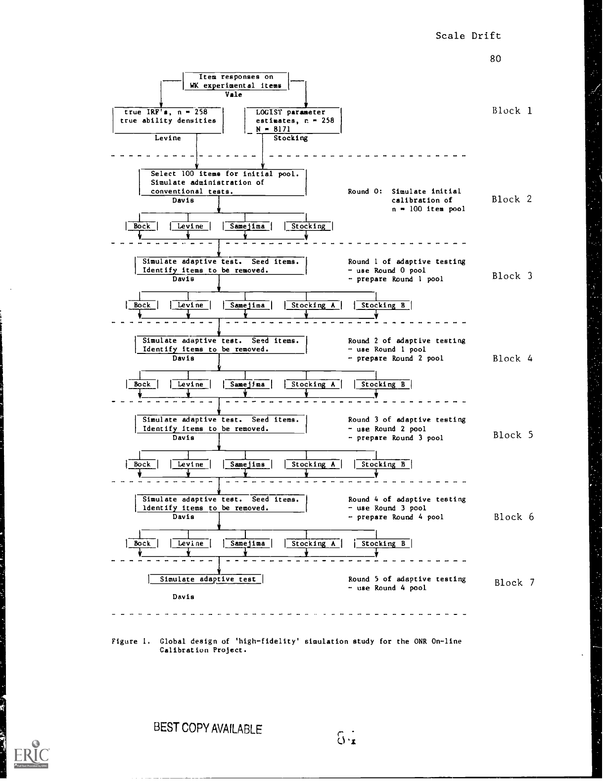
Item responses on
WK experimental items 1---1
Vale
true IRF a, n 258
LOGIST parameter
true ability densities
estimates, n
258
N
8171
Levine Stocking
Scale Drift
Select 100 items for initial pool.
Simulate administration of
conventional tests.
Davis
1
, JL____
1 Bock
1
1
Levine
1
1_1111,11
1
Stocki
1
Round 0: Simulate initial
calibration of
n . 100 item pool
Simulate adaptive test.
Seed items. 1 Round 1 of adaptive testing
Identify items to be removed. - use Round 0 pool
I
Davis
- prepare Round
1 pool
____I____
1
1 Bock 1 1 Levine I
1 Same ima 1 1 Stocking A 1 1
Stocking B
1
-1---
,i
i
I Simulate adaptive test. Seed items. I Round 2 of adaptive testing
Identify items to be removed.
- use Round 1 pool
Davis
1
- prepare Round 2 pool
1 Bock 1 1 Levine 1 Same lea
I I
Stocking A
1 1 Stocking B 1
ISimulate adaptive test. Seed items.
Identify items to be removed.
Davis
Round 3 of adaptive testing
- use Round 2 pool
- prepare Round 3 pool
1
1 Bock Levine
I
Sameijima 1
I
Stocking A 1 1 Stocking B 1
Simulate adaptive test. Seed items.
Round 4 of adaptive testing
Identify items to be removed.
use Round 3 pool
Davis
- prepare RourW 4 pool
____L
1 Bock 1 1
Levine 1 1
Sam:ens/2_ 1
I
Stocking A
Stocking B 1
1 Simulate adaptive test 1 Round 5 of adaptive testing
- use Round 4 pool
Davis
Figure 1.
Global design of 'high-fidelity' simulation study for the ONR On-line
Calibration Project.
BEST COPY AVAILABLE
80
Block 1
Block 2
Block 3
Block 4
Block 5
Block 6
Block 7

0
Scale Drift
81
0
3
-3
-3
0
0
0
0
I 2 I
3
3 -3
0
3
3
3
*
120
0
26
Figure 2.
'True' nonparametric item response functions for some
typical items.
3

Scale Drift
82
0
-3
S CH
1
7b
3
-3
5 CH
*
77
3
3
Figure 3.
Estimated and obseived iLem response functions from
simulated adaptive test responses.

41r-
Method A
Simulate adaptive
test using Round 0 pool.
Identify 25 items to be
removed.
N 4 15000
Seed 50 new items.
5 itess/pereon.
N 1500/1tem
Seed 25 anchor items.
5 iteasiperson.
N
3000/item.
Method B
Compute 8'81
1Fix e s,
calibrate'
new items
'Select 25 replacementl
licema
----4.1Compute 8's]
I
1Fix O's, calibrate new
1
itess
lus anchor items
Ir
Round 1: Use Round 0 poo1;
prepare Round
i pool.
!Transform to
Round 0 scale
iSreelpel:teer2a:nt
Recast
-41
Simulate adaptive
test.
Identify items.
Seed new items.
1Compute 8'81
Ifix 0.0, calibratel
new items
ISelect
re lacementsl
Simulate adaptive test
Identify items.
Seed new items.
Seed anchor items.
"Compute
P.x Vs, calibrate new
items,plus anchor items
!Transform
1St:PI:Cemented
Round 2: Use Round
I pool;
prepare Round 2 pool.
-41
Simulate adaptive
test.
Identify items.
Seed new items.
1Compute ;'s1
1Fix 0 s, calibraeel
new items
11,
'Select
re le:cements'
Simulate adaptive teat.
Identify items.
Seed new items.
Seed anchor items.
'Compute .0.'s1
IFix ;I's, calibrate new
items
lus anchor items
IP
ITransform
I
!Select
Ire lacements1
Round. 3: Use Round 2 pool;
prepare Round 3 pool.
1
1
1
1
Select
Irelacements1
!
-I
Simulate adaptive
test.
Identify items.
Seed new items.
'Compute B's1
1Fix 0 s, calibratel
new items
/
1Sreelpet
l:cementsi
Simulate adaptive test.
Identify items.
Seed new items.
Seed anchor items.
'Compute 0's1
Ins ;'s, calibrate new
items plus anchor items
'Transform
I
I
adaptive
I test
iSimulate
adaptive
test
I
Round A: Use Round 3 pool;
I
Round 5: Use Round
prepare Round 4 pool.
4 pool.
1
1
Figure 4.
Detailed design of simulation study of two LOGIST-based methods of on-line calibration.
dEST COPY
AVAILABLE

RD
i
ARILS
RD 2A ABILS
Rn 3A ARILS
RO AA ARILS
00
cA 491L',
0,1WILFS
Or
RD
RD
RC
Po
PO
pn
O ITEM POO,
C ITEM POOL
O ITFM POOL
O IrEM POOL
C IIEM POCL
LI
e
O 0 0
RD
ABILS. RD 0 ITEM PC01.,
RD 2' ABILS
RD 0 ITEM PCOL
RD 3A ABILS
RD 0 ITEm POCL
RD an ABILS
RD C :*Ey POOL
RO 5n ABILS
RD C ITEm POOL
0,INTILES CW RD 5A r' CISIL
30 AU
50
EC
'POI- SCORE ON
Figure 5.
For all Rounds of Method A, conditional RMSE (left)
and
conditional bias (right) of estimated true score on
the 100-item reference test composed of
Round 0 items.
Dashed vertical lines mark quintiles of
the distribution
of true scores for the final Round.
.)0
13C

C
.;
44-44.-1.4
RD 'SR
G--or--.6
;40 48 .= -s
00
CF
R2 0 I'LM .00-
PD C I'EM
CrL
RD C :-Em PC/-L
70 3 !TEM
pp 0 ITEM POOL
PO 5A XI CISTN
RO
,kBILS
PC 0 ITEm POO.
Ro ze ABILS
RD C ITEM POOL
PC 30 ,,BILS. RD 0 ITEM POOL
PO 4e *OILS
RC 0 ITEM POOL
PG 5e
BI..S
PO C.,
ITEM POOL
GUINTI-ES OF PL
Y: DISTN
:1
--1-
1
4L;
TRUE
SO
SCORE ON
i30
eb
;'EMS
cj
di0
30 WO
2 0
310
1
50 50
TRUE SCORE ON 100 ITEMS
Figure 6.
For all Rounds of Method B, conditional RMSE (left) and
conditional bias (right) of estimated true score on
the 100-item reference test composed of Round 0 items.
Dashed vertical lines mark quintiles of the distribution
of true scores for the final Round.
t3EST COPY AVAb
ANLE
1
70
BO
910
100

-
RD 5A ABILS RD 0 ITEM POOL
0-0-0 RD 58 ASILS
RD 0 ITEM POOL
m-
7
0
Lu
N-1
U.) I
CC
cr
tD
t,1
jtf
o
1
0
Li
-
20
RD 5).
ABILS. RD 0 ITEM POOL
0-61--e
RD 58 ABILS. RD 0 ITEM POOL
ce,
10
i
f
1
4C 50 60
TRUE SCC°F. ON 100 ITEMS
70
80
90 100
20
30 40
50
60
TRUE SCORE ON t00 ITEMS
Figure 7.
After all Rounds for both Methods, conditional RMSE (left)
and conditional bias (right) of estimated true score on
the 100-item reference test composed of Round 0 items.
Dashed vertical lines mark quintiles of the distribution
of true scores for the final Round.
7C
0 910
CO
100

3
5 C H
OH
3
5 C H
#
I 6
3
C H
1
0 -1
5 C H
3
-3
5 C 1-4
oH
3
-3
5 H
Scale Drift
87
#
1 2 1
0
#
2 3
r-
--r
0
#
1 2h
-
3
3
Figure 8.
Typical item response functions estimated by LOGIST (dotted
lines) and the corresponding true item response functions
(solid lines).
Both estimated and true IRF's are on the scale
of the Round 0 pool.

0
0
!
7(
Zi
I
.11 .!
1
-
1
Z.( Z.
I
'
,t
7)
9u
2
o
H
< c\J
H
-
I-
1
0 0
i
0
1
9
11.1
1
-
c.
!
0
I
a_
Z(
1
)
x
Z.(
,?_
)
11
RHO
-
1
)
Z(
1 )
(
1
RHO )
X Z(
)
Figure 9.
Four hundred random draws from a bivariate normal distribution (left),
conditional bias function (middle), and conditional error function (right).
soe
text.
BEST COPY AVAILABLE

residual slopes for
starting pool
--
POINTS NOT PLOTTED
+4. (-7.00.-4.81)
(-8.77.-5.23)
(-5.08.-2.18)
(-3.50.-1.28)
-4
-2
0 2
MEDIAN THAT
approximate error in
estimated abilities
residual difficulties for
starting pool
residual slopes for
new items
Ft
4+44 +I 1+44 1144:14+44.4.
-4 -2
0
2
MEDIAN TTRANS
approximate bias in
estimated abilities
+ +
+
SHAT >- S
0 0 0
SHAT < S
4
Ei
residual difficulties for
new items
Figure 10a.
Snapshot for Method A, Round 1.
See text.

++
+
++
+
+
+
+
+
44t4
+ ++
0
4.*441++
-Ft
t
+
4fr
++
<
+
I
(4
4,
+
1
0 0
0.5
residual slopes for
starting pool
I
0
residual difficulties for
starting pool
< 0
44.+44++++1-+++
o
M
++ POINTS NOT PLOTTED
(-7.00,-4.95)
(-8.52.-3.88)
(-4.94.-2.59)
X
(-3.93.-3.83)
-4
-2 0
2
4
0 0
MEDIAN THAT
approximate error in
estimated abilities
U
0.5
residual slopes for
new itesms
.1 0
-4 -2
0
2
MEDIAN TTRANS
approximate bias in
estimated abilities
-4
-2
0
8
residual difficulties
new items
2
Figure lOb.
Snapshot for Method A, Round 2.
See text.
4
for
.
1
U

residual slopes for
starting pool
POINTS NOT PLOTTED
(-7.00.-5.38)
( 3.82.1.62 )
-2
0
2
MEDIAN THAT
approximate error in
estimated abilities
8
residual difficulties
starting pool
o
o
sr
1
0 0
for
+.41-
++ tH-+
0.5
residual slopes
new items
for
1
0
-4 -2
0
2
MEDIAN TTRANS
approximate bias in
estimated abilities
+
+
SHAT >- S
O
0
0
SHAT < S
0
%+
0 AID
0
0 co
0
0:16
0
0 POINTS NOT PLOTTED
(-2.63.-3.83)
0 (-2.88.-4.05)
1
-4
-2
0
8
residual difficulties
new items
Figure 10c.
Snapshot for Method A, Round 3.
See text.
for

1
4.
residual slopes for
starting pool
+
+
44+4444+4
or
POINTS NOT PLOTTED
+ (-7.00.-4.86)
(-5.21.-2.27)
-7-
I
-4
-2
o
a
MEDIAN THAT
approximate error in
estimated abilities
10
0
0
+
+ 0
,-
4
.
'011N
0
4
+
4 +
SHAT >- S
0 0
0
SHAT < S
-
I
2
2
4
residual di.'ficuldes for
startiAg pool
0.5
residual slopes for
new items
I 0
."4"44+4+4++.1++14.4.
+
FLo
00439
0
00
+
+
+
SHAT >- S
0 0
0
SHAT < S
4
-2
0
2
MEDIAN TTRANS
approximate bias in
estimated abilities
4
residual difficulties for
new items
Figure 10d.
Snapshot for Method A, Round 4.
See text.

0 0
lOu
0.5
residual slopes for
starting pool
1
. 0
++
4.4444-4444:04
+++1.
+44+44+
POINTS NOT PLOTTED
+
(-7.00.-4.81)
(-4.22.-1.82)
(-3.83.-1.18)
4
-2 0 2
MEDIAN THAT
approximate error in
estimated abilities
4
0
+
+
+
SHAT
S
0
0
0
SHAT < S
1 I
-4
-2 0
residual difficulties for
starting pool
1
2 4
i++
4*40*
-4
1
-2 0 2
MEDIAN TTRANS
approximate bias in
estimated abilities
Figure 10e.
Snapshot for Method A. Round 5.
See text.

1
++
. +
- +
+ +
++ -0-
+
+144
il.
+
1- 6
1-
1 o
<
$
+ 4
<
m
I
(4
+
m
0 0 0.5
residual slopes for
starting pool
I
0
1-
POINTS NOT PLOTTED
(-7.00,-4.81)
(-6.77,-5.23)
(-5 06.-2.19)
(-3.50,-1.28)
---T-
1
-4
-2 0 2
4
MEDIAN THAT
approximale error in
estimated abilities
+
+ +
SHAT >- S
0 0 0
SHAT < S
-4
-2
residual difficulties
starting pool
.cr
for
+-4.
0 0
residual slopes for
new items
I 0
0
-4 -2 0
2
MEDIAN TTRANS
approximate bias in
estimated abilities
residual difficulties for
new items
Figure lla.
Snapshot for Method A, Round I.
See text. IOu

1
if
residual slopes for
starting pool
POINTS NOT PLOTTED
(-7.00.-4.87)
(-5.54.-4.52)
(-3.92.-1.28)
1 I
4
2 0
2
MEDIAN THAT
approximate error in
estimated abilities
4
+ +
*
SHAT > S
O 0
0
SHAT < S
residual difficulties for
starting pool
c)
co)
1
0 0
+
+
*
+++ +
I
4.
+
+
+++
+
+
+
.0
+
+
++
+
1
0.5
residual slopes
new items
for
1 0
MEDIAN TTRANS
approximate bias in
estimated abilities
+
+
+
SHAT
S
o
0
0
SHAT < S
POINTS NOT PLOTTED
(-2.93.-1.44)
residual difficulties for
new items
Figure llb.
Snapshot for Method B, Round 2.
See text.

residual slopes for
starting pool
4414++
POINTS NOT PLOTTED
+
+
(-7.00.-5.14)
(-5.35,-2.93)
(-3.96.-1.31)
(-3.51,-1.28)
1
-4
-2
0
2
MEDIAN THAT
approximate error in
estimated abilities
+ +
SHAT >- S
O 0 0
SHAT < S
residual difficulties
starting pool
for
4
+
+
+
+
o
++4+
+
4*
1+ t if+++
H
+-
<
+
++
T
++
++
+ +
+
0.0
1
0.5
residual slopes for
new items
1
H 0
-4
-2
0
2
MEDIAN TTRANS
approximate bias in
estimated abilities
+
+ +
SHAT
>- S
0 0
0 SHAT
< S
POINTS NOT PLOTTED
(-2.88.-1.60)
1
0
-4
residual difficulties for
new items
-2
2
Figure lie.
Snapshot for Method B, Round 3.
See text.
4

residual slopes for
starting pool
44±
POINTS NOT PLOTTED
(-7.00.-4.94)
(-5.32.-2.53)
(-5.10.-3.21)
(-3.99.-1.05)
-4
-2 0
2
MEDIAN THAT
approximate error in
estimated abilities
residual difficulties for
starting pool
residual slopes for
new items
-4
-a 0
2
MEDIAN TTRANS
approximate bias in
estimated abilities
+
+
+
SHAT
>- S
0
0
0
SHAT
< S
0
POINTS NOT PLOTTED
(-2.72.-1.17)
(2.42,3,81 )
-4 -2
2
residual uifficulties for
new items
Figure 11d.
Snapshot for Method B, Round 4.
See text.

0
residual
slopes for
starting pool
POINTS NOT PLOTTED
(-7 00.-5.35)
(-4 09.-2 46)
(-3 89.-1.21)
i
1
I
1
-4 -2
0
2
MEDIAN THAT
approximate error in
estimated abilities
+ +
+
SHAT >- S
0 0
0
SHAT < S
residual difficulties for
starting pool
MEDIAN TTRANS
approximate bias in
estimated abilities
Figure lle.
Snapshot for Method B, Round 5.
See text.
I

Residual Slopes
Residual Difficulties
4.
lzkleA+,4t*
.
0.$ I 0
00
0.$
I 0
0
I 0
0 0
MAT > 2
SHAT < 2
a
Scale Drift
Approximate Bias
in Estimated
Abilities
**14114,,..
04 4/46.
IL
0 0
MOOSAM 17*ANS
-e
m01 AN TYROS
1-
i
0"440"*""%k4
4«
I
I 1
-4 0 p
OM 17011J12
99
Round 1
Round 2
Round 3
Round 4
Round 5
Figure 12.
For all Rounds of Method A, the residuals for the slopes and
the difficulties for items in the starting pool and the
approximate bias in the estimated ability.
See text.
4_0

Residual Slnpes
Residual Difficulties
a
0 0
I 0
1
00
0 0
I 0
0 0
I
>.
0
0
0 MAT
Scale Drift
Approximate Bias
in Estimated
Abilities
°
1
-t 0
INDIAN 11114166
----T
-4
-0
0
8$01
TTRAWS
7
+4414114.44.
44.441.04.0.
-e
0
t
VIE014.14 TTRAlts
100
Round I
Round 2
Round 3
Round 4
Round 5
Figure 13.
For all Rounds of Method
B, the residuals for the
slopes and
the difficulties for items
in the starting pool and the
approximate bias in the estimated
ability.
See text.

Approximate Error
in Estimated Abilities
'No*
TOMS MOT PLOTTIO
1
-4 00. -4 .01
1
1
04. -t IS
-11.110.-1.24
1
1
1
-t 0 Z
MEDIAN MAT
TO14TI MOT PLOT=
I -7 . 00 . -0 20 1
Git .1. St 1
Scale Drift
Residual Slopes
Residual Difficulties
0 0
'!
0 0
.:1114,4 +++-
4:
0 . 6
4. 4+
-4
D 0
0
0
I 0
SHAY
111
0 0 0
SKIT
101
Round 1
Round 2
Round 3
Round 4
Round 5
Figure 14.
For all Rounds of Method A, the approximate error function for
the estimated abilities and the residuals for the slopes and
difficulties for the new items.
See text.
u

Approximate Error
in Estimated Abilities
POINTS NOT PLOTTED
1-7.00.-4.11 1
1-4.00.-0. IS 1
1 -3.40.-1.26 1
-4 -t
0
0
WOTAN THAT
POINTS 1404 ruorrso
-7 .00 . -4.47 1
44.14 . -4Si /
300 -1 1111
-4
-It 0 0
4
MIT NI THAT
POINTS ler H.orrro
1-7.00.-41.141
1-S.34.-0.63 1
1 -3.96. -1.31 1
1
-t 0
2
INDIAN THAT
POINTS MT PLOTTED
-7. 00. -4. 64 1
1-9.10.-3.01 1
1-3 .11 . -1.06 1
-r o
0
o o
1460141 THAT
Scale Drift
Residual Slopes
Residual Difficulties
49d,
:7
+,
0 9
0 0
1 0
lb
-'4+*!: 444
+ 47.t.;
4+6 +
0 0 0.1
1
0
+i *+
ttt4:-+
44.44.
POINTS NOT PLOTTIO
1 -7.03.-4.01
1-4 NE -0 . 1
1-3.111.-1./11
--1
-I
0
0
11110144 THAT
0.5 1
0
V
SHAT >
O
0 0
1144iT <
0
0 0
POIXTS NOT PLOTTIM
I
-a .63.-1.44 1
4011440 NOT 41.011112
1 -0 1141. -1 . CO 1
0
POINTS NOT P1.01-4113
-t Pi . -1. /7
I. 44 . 3 .1 I
1
-4
0 &
102
Round 1
Round 2
Round 3
Round 4
Round 5
Figure 15.
For all Rounds of Me..thod B, 'the approximate error function for
the estimated abilities and the residuals for the slopes and
difficulties for the new items.
See text.
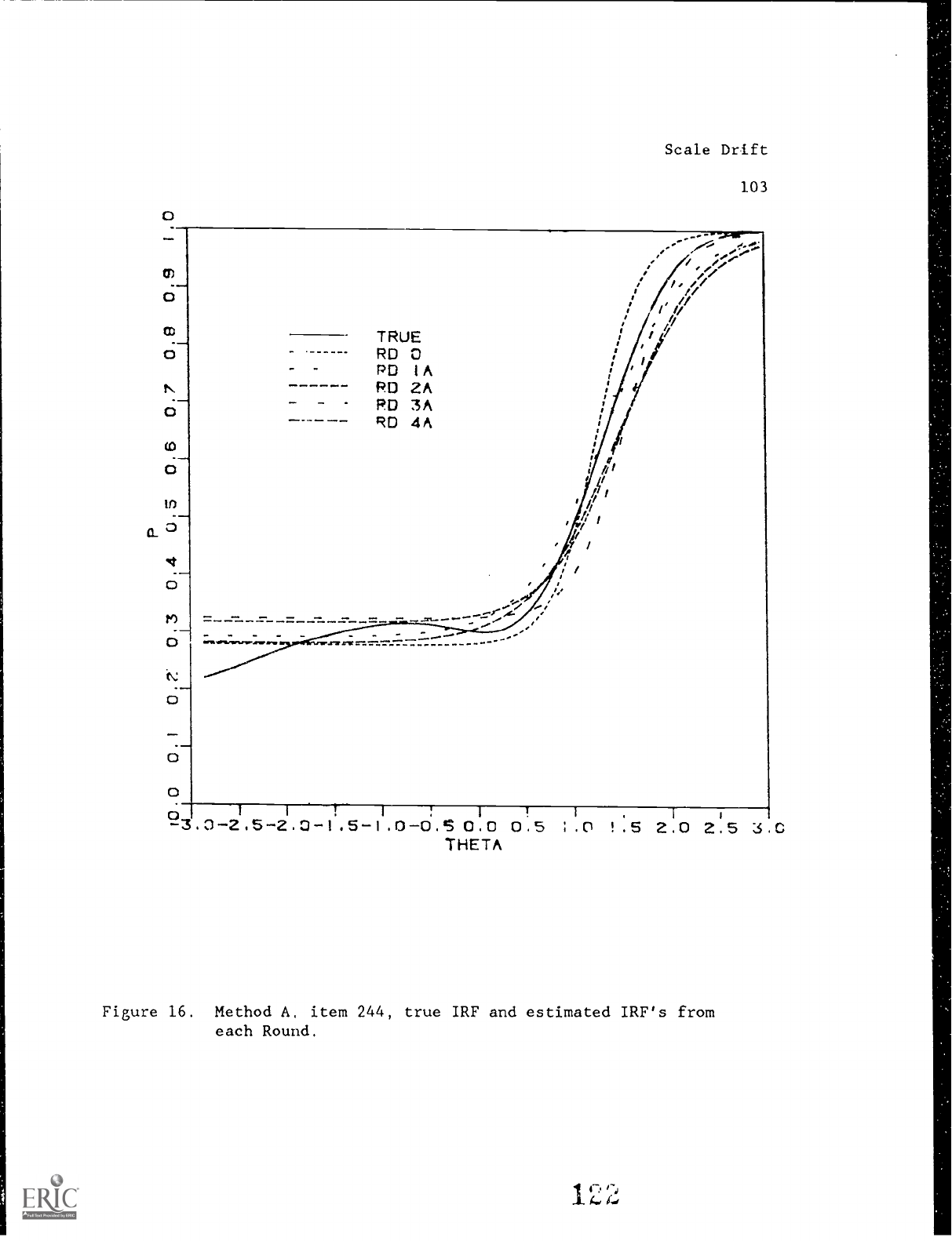
0
Scale
Drift
103
a
3
TRUE RD
0
PD
I
A
RD
ZA
RD
3A
RD
4A
0
3.0-2.5-2.0I
.5I
.0-0.S
0.0
O.
5
!
5
2.0
2.5
3
C
THETA
Figure
16.
Method
A,
item
244,
true
IRF
and
estimated
IRF's
from
each
Round.
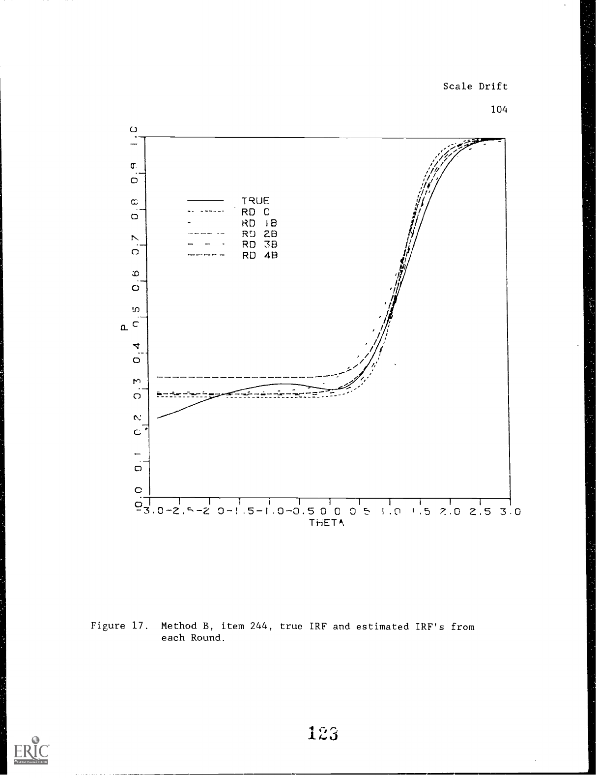
0
0
0
N.
0
C.
Scale Drift
104
TRUE
(//
-----
RD 0
RD I
RD
28
RD 38
RD
48
---------------------
.0.
II
II
c
0
1 1 1 i
1 1
1
I
I I
1
-3.0 -2.'s-2 0-L5-1.0-0.50 0 0 5
1.0
1.5 7..0 2.5 3 0
THETo
Figure 17.
Method B, item 244, true IRF and estimated IRF's from
each Round.

Residual Slopes
0 0
0.5
I C
0 0
0.5
I
0
Scale Drift
Residual Difficulties
+
+ + SHAT
>- S
0 0
0
SHAT < S
m
Method
I
o
t--.
<
I
A
m
Method
before
scaling
o
0
0
0
0
+F d OD+
+
o
o
64?
o o
+
0
-4
-2
0
2 4
Method
1
after
scaling
105
Figure 18a.
The Round 1 residuals for the slopes and difficulties for new items
for Method A (top), Method B before scaling (middle), and Method B
after scaling (bottom).
See text.
2 4

Residual Slopes
m
iTO
Ht o
<
Method
<
i
i
(4
A
m
vr
0 0 0.5
1 0
0 0
0.5
1 0
Scale Drift
Residual Difficulties
+
+ +
SHAT
>- S
0 0
0 SHAT
< S
0
Method
before
scaling
Method
after
scaling
POINTS NOT PLOTTED
(-2.93.-1.90)
+
00
;-84"-imezr0
+
0 +
0 0
oo
0
0
106
-4
-2
2
POINTS NOT PLOTTED
(-2.93.-1.44)
4
-4 -2
Figure 18b,
The Round 2 residuals for the slopes and difficulties for new
items
for Method A (top), Method B before scaling (middle), and
Method B
after scaling (bottom) .
See text.
:3

0
Residual Slopes
0 0
1
0.5
Method
A
Scale Drift
Residual Difficulties
+ +
+
SHAT
>- S
0 0 0
SHAT < S
POINTS NOT PLOTTED
(-2.63,-3.63)
(-2.88,-4.05)
o
06.aa
o
o v
1
1
-4
-2 0
4
0
I o
H
Method
before
scaling
Method
after
scaling
0
107
POINTS NOT PLOTTED
(-2.88,-2.10)
-2
0 2 4
POINTS NOT PLOTTED
(-2.88,-1,60)
0
+0
00 0
-4 -2
Figure 18c.
The Round 3 residuals for the slopes and difficulties for new items
for Method A (top), Method B before scaling (middle), and Method
B
after scaling (bottom).
See text.
12u

o
o
Residual Slopes
0 0
1
0.5 1 0
f--1 0
Method
A
a)
Method
before
scaling
Scale Drift
Residual Difficulties
+
+ +
SHAT
>- S
0 0
0
SHAT
< S
POINTS NOT PLOTTED
(-2.72,-1.49)
(2.42,4.40)
1 o
Method
after
scaling
POINTS NOT PLOTTED
( -2.72. I .171
( 2.42.3.81)
-2
0
2
4
08
Figure 18d.
The Round 4 residuals for the slopes and difficulties for new items
for Method A (top), Method B before scaling (middle), and Method B
after scaling (bottom).
See text.
el*'
4, I

TEST I
50.0
317.5
25.0
12.5
o
-.....
RoLva
a
-
.r.:
..re-
-a-
^ d-
.,.
fliPal'ea-:NN%-
'"*.,..,
-+N.
\
'\,,..,....
\
-VD
Scale Drift
\
/-
i
/
r5
,.
b,
"...
ft ,.i'
.69' ..
ir".
.\
. : b :
,,s9 ..'
;'.
NY
....
..-' ,
0 ..
i
3,0
1.5
Ro un d 4
THETA
+1.5
109
Figure 19.
Method A estimated test information functions for the 100-item
pools at each Round of simulations.

TEST I
50.0
37.5
25.0
12.5
Scale Drift
110
re%-
de"
un d 4
-3.0 -1.5
THETA
+1.5
Figure 20.
Method B estimated test information functions for
the 100-item
pools at each Round of simulations.

TEST I
40
30
20
10
MEM
-3.0
Scale Drift
111
50 new it.--
25 rep lacemen t items
-N-
1
-1.5
THETA
Figure 21.
Method A estimated test information functions for the target,
the 50 new items and the 25 replacement items, Round 4.

TEST I
40
30
20
10
-3. 0
50 new items
Ka.
MONO
VAIL.e.e"'
25 replacement items
Scale Drift
"s4k-..
1
-1.5
112
1114.1
+1.5
+3.
THETA
Figure 22. Method B estimated test information functions for the target,
the 50 new items and the 25 replacement items, Round 4.
101

Scale Drift
113
Appendix 1.
Parameter estimates for items not included in Figures becau!-;e
'true' parameters could not be developed from the tabled
values of the true item response functions
Figure Row
Column
a
10a 1
1,2
.87
-3.94
.07
.70 3.92
.10
1.03 -3.45
.07
.88 -3.72
.07
2.11 10.18
.22
2
2,3 .31 -11.07
.20
.54
-4.13 .20
.99
-3.17
.20
.32
-8.85
.20
1.10
-3.20
.20
.21 -9.82
.20
.90 -2.79
.20
.68 -3.86
.20
.41 -6.54
.20
.13 -14.88
.20
10b 1
1,2
.87 -3.94
.07
.70 3.92
.10
1.03 -3.45
.07
.88
-3.72
.07
2.11
10.18
.22
2
2,3 .76
-5.22
.20
1.01 -3.00
.20
.65 -2.78
.20
.50 -5.88
.20
1.05 -2.83
.20
.41 -6.57
.20
.28
-10.88
.20

Figure
Scale Drift
114
A
Row-
Column a
10c 1
1,2
.87
-3.94
.07
.70 3.92
.10
1.03 -3.45
.07
.88
-3.72
.07
2.11
10.18
.22
.65 -2.78
.20
2
2,3
.89
-3.26
.20
.05 -66.42
.20
.60 -3.34
.20
.66 -3.92
.20
1.21 2.83
.10
.50 -5.46
.20
.34 3.46
.20
1.08
-3.35
.20
.57 -3.55
.20
.65 -3.87
.20
10d
1
1,2 .87
-3.94
.07
.70 3.92
.10
1.03
-3.45
.07
.88 -3.72
.07
2.11 10.18
.22
.65 -2.78
.20
2
2,3
.44
-5.94
.20
.40 -6.89
.20
1.04 -3.14
.20
1.42 -3.37
.20
.51 -5.32
.20
1.10
-3.11
.20
.61
-4.21
.20
2.02
3.02
.19
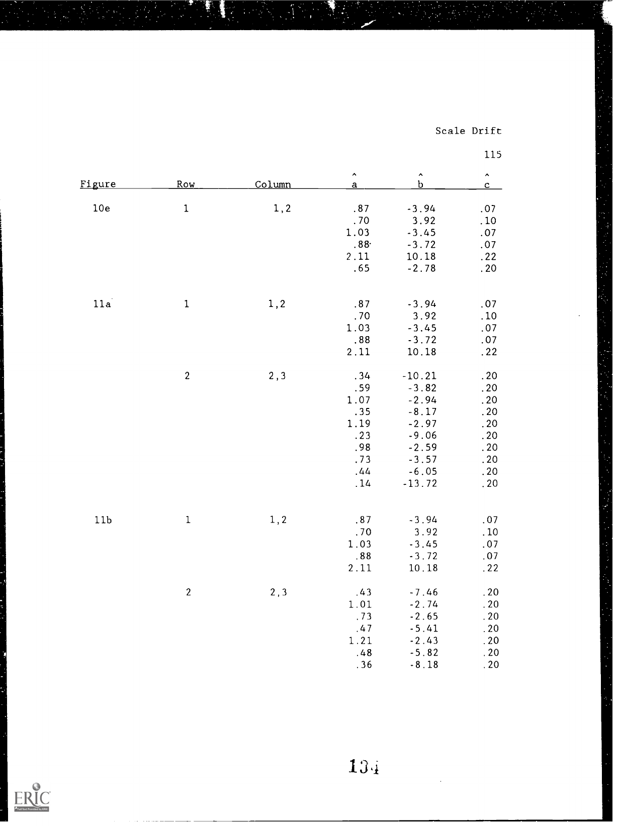
...
Scale Drift
115
A
A
Figure
Row Column
a
b c
lOe 1 1,2 .87
-3.94
.07
.70
3.92 .10
1.03 -3.45
.07
.88. -3.72 .07
2.11 10.18 .22
.65
-2.78
.20
lla 1 1,2 .87
-3.94
.07
.70 3.92 .10
1.03 -3.45 .07
.88 -3.72
.07
2.11 10.18 .22
2 2,3 .34 -10.21 .20
.59 -3.82 .20
1.07 -2.94 .20
.35 -8.17
.20
1.19 -2.97 .20
.23 -9.06 .20
.98 -2.59 .20
.73 -3.57 .20
.44
-6.05 .20
.14 -13.72 .20
llb
1 1,2 .87
-3.94 .07
.70 3.92 .10
1.03
-3.45 .07
.88 -3.72 .07
2.11 10.18 .22
2
2,3
.43
-7.46
.20
1.01
-2.74
.20
.73 -2.65
.20
.47
-5.41
.20
1.21 -2.43
.20
.48
-5.82
.20
.36 -8.18 .20
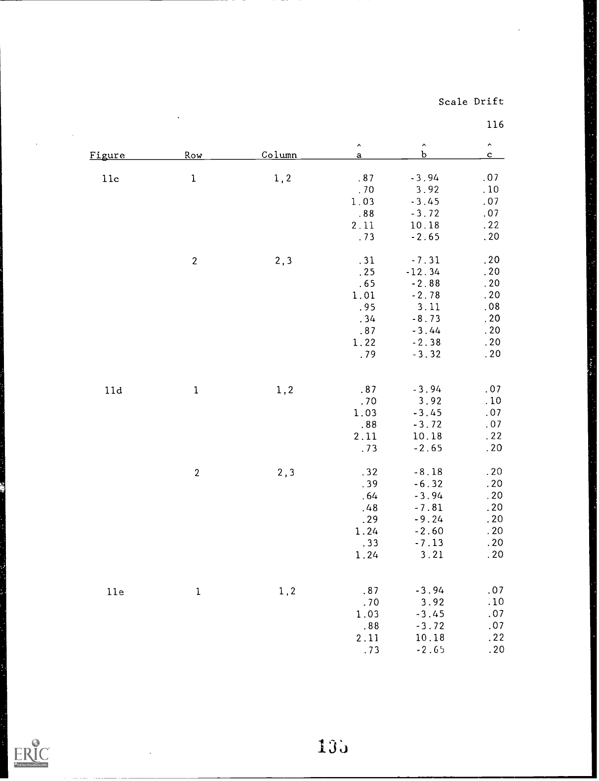
Scale Drift
116
Figure Row
Column
a
11c
1
1,2 .87
-3.94 .07
.70
3.92
.10
1.03
-3.45 .07
.88
-3.72 .07
2.11 10.18
.22
.73 -2.65
.20
2
2,3 .31
-7.31
.20
.25
-12.34
.20
.65
-2.88
.20
1.01 -2.78
.20
.95
3.11
.08
.34 -8.73
.20
.87
-3.44 .20
1.22 -2.38
.20
.79
-3.32
.20
lld
1
1,2
.87
-3.94 .07
.70
3.92
.10
1.03
-3.45 .07
.88
-3.72
.07
2.11 10.18
.22
.73
-2.65 .20
2
2,3 .32
-8.18 .20
.39
-6.32
.20
.64
-3.94 .20
.48
-7.81
.20
.29
-9.24 .20
1.24
-2.60
.20
.33
-7.13 .20
1.24
3.21
.20
lle
1
1,2
.87
-3.94 .07
.70
3.92 .10
1.03
-3.45 .07
.88
-3.72 .07
2.11
10.18 .22
.73
-2.65 .20
13:)
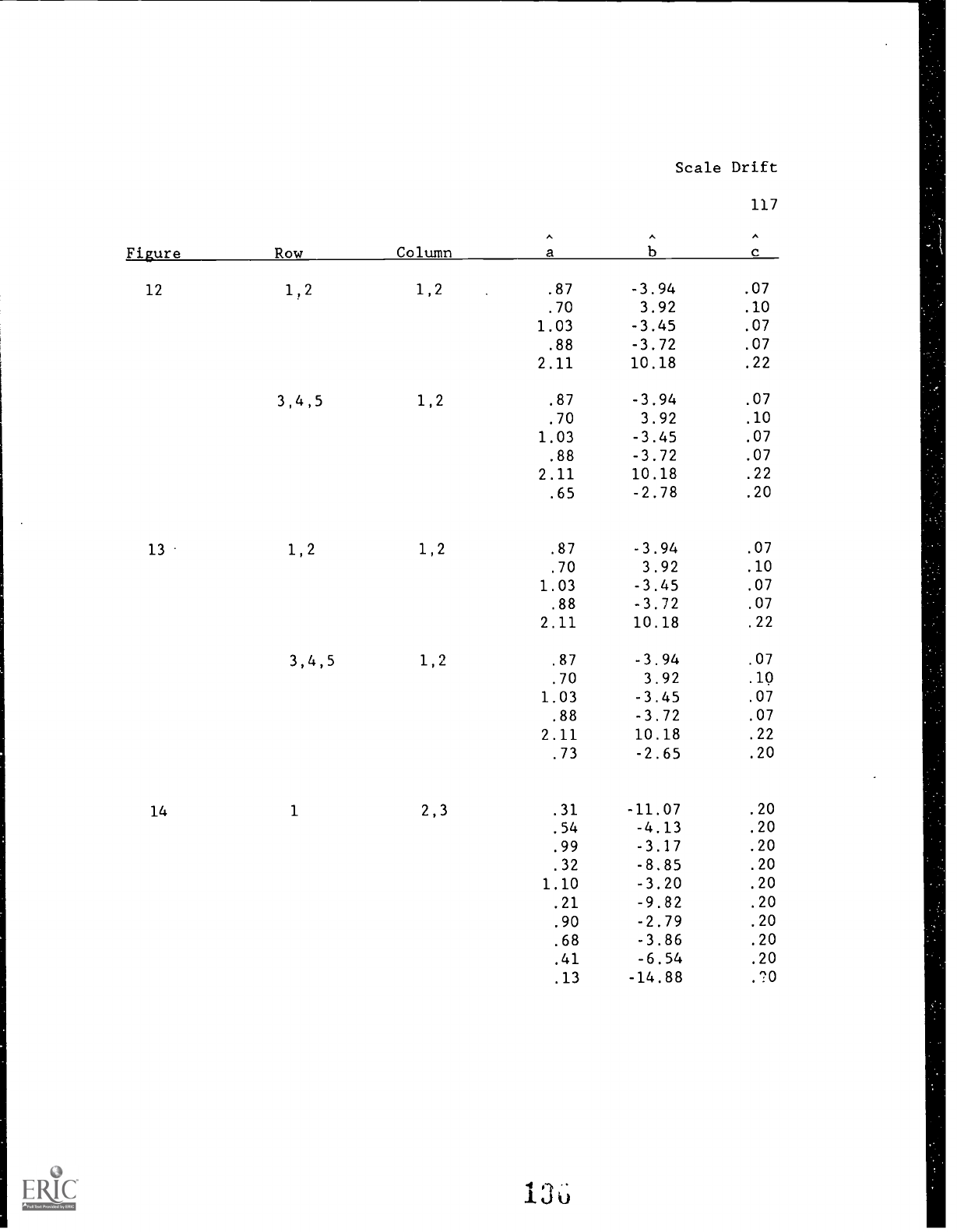
Figure
Row
Column
A
a
Scale Drift
117
A
A
12 1,2
1,2
.87
-3.94
.07
.70
3.92
.10
1.03
-3.45
.07
.88
-3.72
.07
2.11
10.18
.22
3,4,5
1,2
.87 -3.94
.07
.70
3.92
.10
1.03
-3.45
.07
.88 -3.72
.07
2.11
10.18
.22
.65
-2.78
.20
13
1,2
1,2 .87
-3.94
.07
.70
3.92
.10
1.03
-3.45
.07
.88 -3.72
.07
2.11
10.18
.22
3,4,5
1 2,
.87 -3.94
.07
.70
3.92
.10
1.03
-3.45
.07
.88 -3.72
.07
2.11
10.18
.22
.73
-2.65
.20
14
1
2,3
.31
-11.07
.20
.54
-4.13 .20
.99
-3.17
.20
.32
-8.85
.20
1.10 -3.20
.20
.21
-9.82
.20
.90 -2.79
.20
.68
-3.86
.20
.41 -6.54
.20
.13
-14.88
.?0

Scale Drift
118
Figure
Row Column a
14 (cont'd.)
2
3
4
2,3 .76 -5.22 .20
1.01 -3.00 .20
.65 -2.78 .20
.50
-5.88
.20
1.05 -2.83 .20
.41 -6.57
.20
.28 -10.88
.20
2,3 .89 -3.26 .20
.05 -66.42
.20
.60 -3.34 .20
.66 -3.92 .20
1.21 2.83 .10
.50 -5.46 .20
.34 3.46 .20
1.08
-3.35 .20
.57 -3.55 .20
.65 -3.87 .20
2,3
.44 -5.94 .20
.40 -6.89 .20
1.04 -3.14
.20
1.42 -3.37 .20
.51 -5.32 .20
1.10 -3.11
.20
.61 -4.21 .20
2.02
3.02 .19
15 1
2,3 .34 -10.21
.20
.59 -3.82
.20
1.07
-2.94
.20
.35 -8.17
.20
1.19 -2.97
.20
.23 -9.06
.20
.98 -2.59
.20
.73 -3.57 .20
.44 -6.05
.20
.14 -13.72
.20

A
Scale Drift
119
A A
Figure Row
Column
a
b c
15 (cont'd.)
2
3
4
2,3
.43 -7.46
.20
1.01
-2.74
.20
.73 -2.65
.20
.47
-5.41
.20
1.21
-2.43
.20
.48
-5.82
.20
.36 -8.18
.20
2,3
.31
-7.31
.20
.25
-12.34
.20
.65 -2.88
.20
1.01
-2.78
.20
.95
3.11
.08
.34
-8.73
.20
.87
-3.44
.20
1.22
-2.38
.20
.79
-3.32 .20
2,3
.32
-8.18 .20
.39
-6.32
.20
.64
-3.94 .20
.48
-7.81 .20
.29
-9.24
.20
1.24
-2.60
.20
.33
-7.13
.20
1.24
3.21
.20
18a
1 1,2
.31
-11.07
.20
.54
-4.13 .20
.99 -3.17
.20
.32
-8.85
.20
1.10
-3.20
.20
.21 -9.82
.20
.90 -2.79
.20
.68 -3.86
.20
.41
-6.54
.20
.13 -14.88
.20

Figure
Row
18a (cont'd.)
2
18b
BEST COPY AVAILABLE
3
1
2
Column
1,2
1,2
1,2
1,2
133
Scale Drift
A
a
120
A
.31
-11.07
.20
.54
-4.13
.20
.99
-3.17
.20
.32
-8.85
.20
1.10
-3.20
.20
.21
-9.82
.20
.90
-2.79
.20
.41
-6.54 .20
.13
-14.88
.20
.34
-10.21
.20
.59
-3.82
.20
1.07
-2.94
.20
.35
-8.17
.20
1.19
-2.97
.20
.23
-9.06
.20
.98
-2.59
.20
.73
-3.57
.20
.44
-6.05
.20
.14
-13.72
.20
.76
-5.22
.20
1.01
-3.00 .20
.65
-2.78
.20
.50
-5.88
.20
1.05
-2.83
.20
.41
-6.57
.20
.98
-10.88
.20
.39
-8.28 .20
.91
-3.02 .20
.65
-2.92
.20
.42
-6.00
.20
1.08
-2.67
.20
.43
-6.45
.20
.32
-9.09
.20
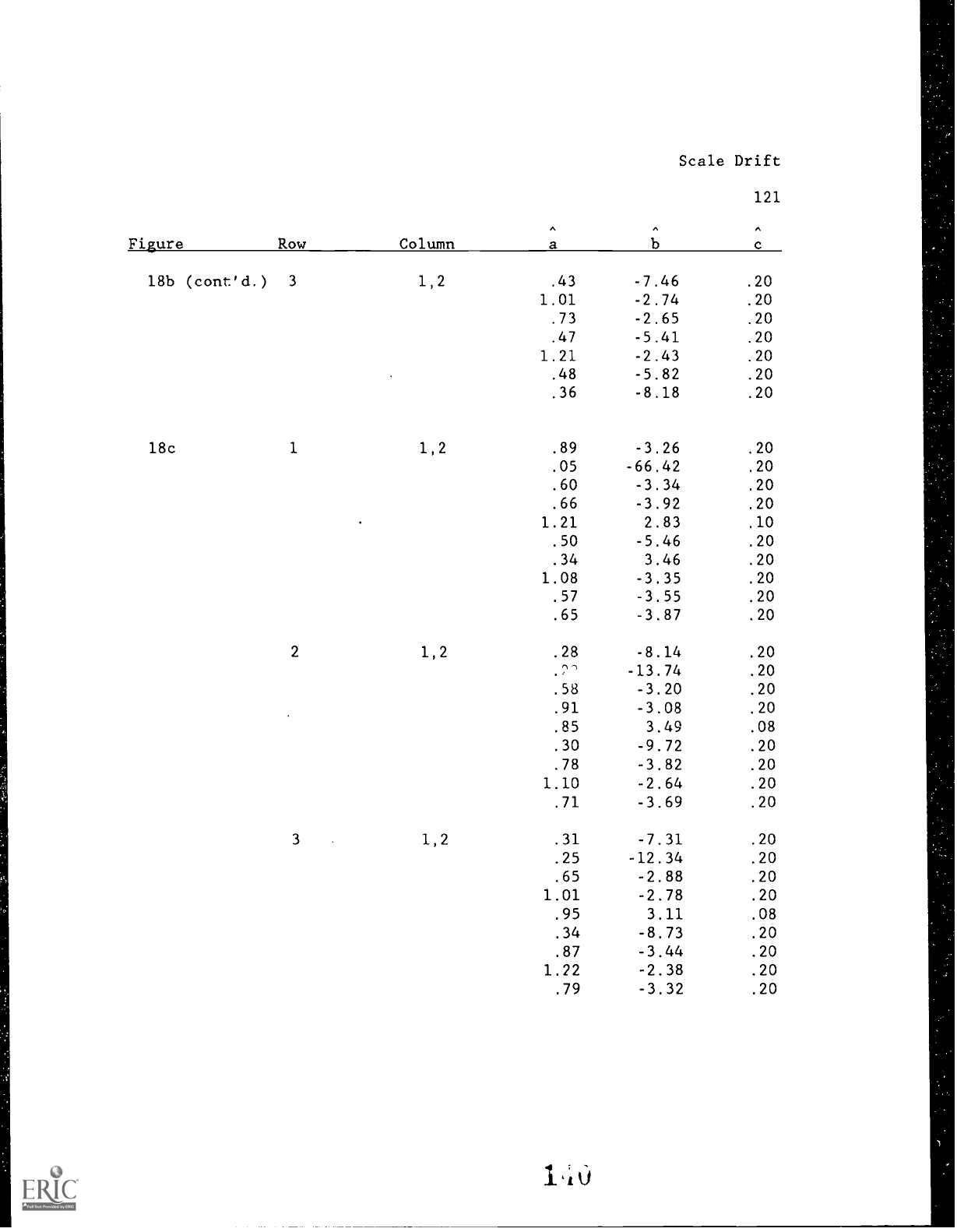
Scale Drift
121
Figure Row Column a b
c
18b (cont'd.) 3 1,2 .43
-7.46 .20
1.01 -2.74
.20
.73 -2.65
.20
.47 -5.41 .20
1.21 -2.43 .20
.48
-5.82 .20
.36 -8.18 .20
18c 1 1,2 .89 -3.26 .20
.05
-66.42
.20
.60 -3.34 .20
.66
-3.92
.20
1.21 2.83 .10
.50 -5.46 .20
.34 3.46 .20
1.08 -3.35
.20
.57 -3.55 .20
.65 -3.87 .20
2 1,2 .28 -8.14 .20
,-,-,
-13.74 .20
.58 -3.20 .20
.91 -3.08 .20
.85 3.49 .08
.30
-9.72
.20
.78 -3.82 .20
1.10 -2.64 .20
.71
-3.69
.20
3 1,2 .31 -7.31 .20
.25 -12.34 .20
.65 -2.88 .20
1.01 -2.78 .20
.95 3.11 .08
.34 -8.73 .20
.87 -3.44 .20
1.22 -2.38 .20
.79 -3.32 .20

Figure
18d
ROW Column
A
a
b
Scale Drift
122
A
1
2
3
BEST COPY
AVAILARLE
1,2
1,2
1,2
.44
.40
1.04
1.42
.51
1.10
.61
2.02
.29
.36
.59
.44
.26
1.14
.31
1.14
.32
.39
.64
.48
.29
1.24
.33
1.24
-5.94
-6.89
-3.14
-3.37
-5.32
-3.11
-4.21
3.02
-8.83
-6.86
-4.26
-8.48
-10.05
-2.81
-7.74
3.53
-8.18
-6.32
-3.94
-7.81
-9.24
-2.60
-7.13
3.21
.20
.20
.20
.20
.20
.20
.20
.19
.20
.20
.20
.20
.20
.20
.20
.20
.20
.20
.20
.20
.20
.20
.20
.20
Educational Testing Service/Stocking
Dr. Terry Ackerman
Dr. R. Darrell Bock
American College Testing Programs
University of Chicago
P.O. Box 168
NORC
Iowa City, IA 52243
6030 South Ellis
Chicago, IL
60637
Dr. Robert Ahlers
Code N711
Human Factors Laboratory
Naval Training Systems Center
Orlando, FL
32813
Dr. James Algina
1403 Norman Hall
University of Florida
Gainesville, FL 32605
Dr. Erling B. Andersen
Department of Statistics
Studiestraede 6
1455 Copenhagen
DENMARK
Dr. Eva L. Baker
UCLA Center for the Study
of Evaluation
145 Moore Hall
University of Californi3
Los Angeles, CA 90024
Dr. Isaac Bejar
Mail Stop: 10-R
Educational Testing Service
Rosedale Road
Princeton, NJ 08541
1986/04/2C
Cdt. Arnold Bohrer
Sectie Psychologisch Onderzoek
Rekruterings-En Selectiecentrum
Kwartier Koningen Astrid
Bruijnstraat
1120 Brussels, BELGIUM
Dr. Robert Breaux
Code 78
Naval Training Systems Center
Orlando, FL 32813-7100
Dr. Robert. Brennan
American College Testing
Programs
P. O. Box 168
Iowa City, IA 52243
Dr. James Carlson
American College Testing
Program
P.O. Box 168
Iowa City, IA 52243
Dr. John B. Carroll
409 Elliott Rd., North
Chapel Hill, NC 2/514
Dr. Robert M. Carroll
Dr. Menucha Birenbaum
Chief of Naval Operations
School of Education
OP-0182
Tel Aviv University
Washington, DC
20350
Ramat Aviv 69978
ISRAEL
Dr. Raymond E. Christal
UES LAMP Science Advisor
Dr. Arthur S. Blaiwes
AFHRL/MOEL
Code N712
Brooks AFB,
rx 78235
Naval Training Systems Center
Orlando. FL 32313-7100
Dr. Norman Cliff
Department of Psychology
Dr. Bruce Bloxom
Univ. of So. California
Defense Manpower Data Center
Los Angeles, CA 90089-1061
550 Camino El Estero,
Suite 200
Monterey, CA 93943-3231
4
dEST COPY AVAILABLE

1988/04/20
Educational lesting Service/Stocking
Director,
Manpower Support and
Readiness Program
Center for Naval Analysis
2000 North Beauregard Street
Alexandria, VA 22311
Dr. Stanley Collyer
Office of Naval Technology
Code 222
800 N. Quincy Street
Arlington, VA 22217-5000
Dr. Hans F. Crombag
Faculty of Law
University of Limburg
P.O. Box 616
Maastricht
The NETHERLANDS 6200 MD
Dr. Timothy Davey
Educational Testing Service
Princeton, NJ 08541
Dr. C. M. Dayton
Department of Measurement
Statistics & Evaluation
College of Education
University of Maryland
College Park, MD 20742
Dr. Ralph J. DeAyala
Measurement, Statistics,
and Evaluation
Benjamin Bldg., Rm. 4112
University of Maryland
College Park, MD 20742
Dr. Dattprasad Divgi
Center for Naval Analysis
4401 Ford Avenue
P.O. Box 16268
Alexandria, VA 22302-0268
Dr. Hei-Ki Dong
Bell Communications Research
6 Corporate Place
PYA-1K226
Piscataway, NJ 08854
Dr. Fritz Drasgow
University of Illinois
Department of Psychology
603 E. Daniel St.
Champaign, IL 61820
Defense Technical
Information Center
Cameron Station, Bldg 5
Alexandria, VA 22314
Attn: TC
(12 Copies)
Dr. Stephen Dunbar
2248 Lindquist Center
for Measurement
University of Iowa
Iowa City, IA 52242
Dr. James A. Earles
Air Force Human Resources Lab
Brooks AFB, TX 78235
Dr. Kent Eaton
Army Research Institute
5001 Eisenhower Avenue
Alexandria, VA 22333
Dr. John M. Eddins
University of Illinois
252 Engineering Research
Laboratory
103 South Mathews Street
Urbana; IL 61801
Dr. Susan Embretson
University of Kansas
Psychology Department
426 Fraser
Lawrence, KS 66045
Dr. George Englehard, Jr.
Division of Educational Studies
Emory University
210 Fishburne Bldg.
Atlanta, GA 30322
Dr. Benjamin A. Pairbank
Performance Metrics, Inc.
5825 Callaghan
Suite 225
San Antonio, IX 78228

1988/04/20
Educational Testing Service/Stocking
Dr. P-A. Federico
Code 51
NPRDC
San Diego, CA 92152-6800
Dr. Leonard Feldt
Lindquist Center
for Measurement
University of Iowa
Iowa City, IA 52242
Dr. Richard L. Ferguson
American College resting
P.O. Box 168
Iowa City, IA 52243
Dr. Gerhard Fischer
Liebiggasse 5/3
A 1010 Vienna
AUSTRIA
Dr. Myron Fischl
U.S. Army Headquarters
DAPE-MRR
The Pentagon
Washington, DC
20310-0300
Prof. Donald Fitzgera.d
University of New England
Department of Psychology
Armidale, New South Wales
AUSTRALIA
Mr. Paul Foley
Navy Personnel R&D Center
San Diego, CA 92152-6300
Dr. Robert Glaser
Learning Research
& Development Center
University of Pittsburgh
3939 O'Hara Street
Pittsburgh, PA 15260
Dr. Bert Green
Johns Hopkins University
Department of Psychology
Charles & 34th Street
Baltimore, MD 21218
DORNIER GMBH
P.O. Box 1420
D-7990 Friedrichshafen
1
WEST GERMANY
Dr. Ronald K. Hambleton
University of Massachusetts
Laboratory of Psychometric
and Evaluative Research
Hills South, Room 152
Amherst, MA 01003
Dr. Delwyn Harnisch
University of Illinois
51 Gerty Drive
Champaign, IL 61820
2351
Dr. Grant Henning
Senior Research Scientist
Division of Measurement
Research and Services
Educational Testing Service
Princeton, NJ
03541
Dr. Alfred R. Freoly
AFOSR/NL, Bldg. 410
Bolling AFB, DC 20332-6448
Dr. Robert D. Gibbons
Illinois State Psychiatric Inst.
Rm 529W
1601 W. Taylor Street
Chicago, IL 60612
Dr. Janice Gifford
University of Massachusetts
School of Education
Amherst, MA 01003
i3EST COPY
AVAILABLE
144
Ms. Rebecca Netter
Navy Personnel R&D Center
Code 63
San Diego, CA 92152-6800
Dr. Paul W. Holland
Educational Testing Service, 21-T
Rosedale Road
Princeton, NJ
08541
Prof. Lutz F. Hornke
Institut fur Psychologie
RW1H Aachen
Jaegerstrasse 17/19
D-5100 Aachen
WEST GERMANY

Educational Testing Service/Stocking
Dr. Paul Horst
677 G Street, #184
Chula Vista, CA 92010
Mr. Dick Hoshaw
OP-135
Arlington Annex
Room 2834
Washington, DC 20350
Dr. Lloyd Humphreys
University of Illinois
Department of Psychology
603 East Daniel Street
Champaign, IL 61820
Dr. Steven Hunka
3-104 Educ. N.
University of Alberta
Edmonton, Alberta
CANADA
T6G 2G5
Dr. Huynh Huynh
College of Education
Univ. of South Carolina
Columbia, SC 29208
Dr. Robert Jannarone
Elec. and Computer Eng. Dept.
University of South Carolina
Columbia, SC 29208
Dr. Douglas H. Jones
Thatcher Jones Associates
P.O. Box 6640
10 Trafalgar Court
Lawrenceville, NJ
08648
Dr. Milton S. Katz
European Science Coordination
Office
U.S. Army Research Institute
Box 65
FPO New York
09510-1500
Prof. John A. Keal:s
Department ot Psvcholonv
Lhiversitv of Newcastlk?
N.S.W. 230U
AUSTRALIA
1988/04/20
Dr. G. Gage Kingsbury
Portland Public Schools
Research and Evaluation Department
501 North Dixon Street
P. O. Box 3107
Portland, OR 97209-3107
Dr. William Koch
Box 7246, Meas. and Eval. Ctr.
University of Texas-Austin
Austin, TX 78703
Dr. James Kraatz
Computer-based Education
Research Laboratory
University of Illinois
Urbana, IL 61801
Dr. Leonard Kroeker
Navy Personnel R&D Center
Code 62
San Diego, CA 02152-6800
Dr. Jerry Lehnus
Defense Manpower Data Center
Suite 400
1600 Wilson Blvd
Rosslyn, VA 22209
Dr. Thomas Leonard
University of Wisconsin
Department of Statistics
1210 West Dayton Street
Madison, WI 53705
Dr. Michael Levine
Educational Psychology
210 Education Bldg.
University of Illinois
Champaign, IL 61801
Dr. Charles Lewis
Educai:ional Testing Service
Princeton, NJ 08541-0001
Dr. Robert L. Linn
Campus Box 24:-1,
Uoiversity of Colorado
Boulder, CO
80309-0249

198,04/20
Educational Festino Service/Stockino
Dr. Pohert Lockman
Cerit.r 'or Naval Analysis
4401 Ford Avenue
P.O. Box 16268
Alexandria, VA 22302-0268
Dr. Frederic M. Lord
Educational Testing Service
Princeton, NJ 08541
Dr. George B. Macready
Department of Measurement
StatistKs & Evaluation
College of Education
University of Maryland
College Park, MD 20/42
Dr. Gary Marco
Stop 31-E
Educational Testing Service
Princeton, NJ 08451
Dr. James R. McBride
The Psychological Corporation
1250 Sixth Avenue
San Diego, CA 92101
Dr. Clarence C. McCormick
HO, USMEPCOM/MEPCT
2500 Green Bay Road
North Chicago, IL 60064
Dr. Robert McKinley
Educational Testing Service
16-T
Princeton, NJ 08541
Dr. James McMichael
Technical Director
Navy Personnel R&D Center
San Diego, CA 92152-6800
Dr. Barbara Means
SRI International
333 Ravenswood Avenue
Menlo Park, CA
94025
Dr. Robert Mislevy
Educational
Festing Service
Princeton, NJ 08541
140
Or. William Montague
NPRDC Code 13
San Diego, CA 92152-6800
Ms. Kathleen Moreno
Navy Personnel R&D Center
Code 62
San Diego, CA 92152-6800
Headquarters Marine Corps
Code MPI-20
Washington, DC 20360
Dr. W. Alan Nicewander
University of Oklahoma
Department of Psychology
Norman, OK 73071
Deputy Technical Director
NPRDC Code 01A
San Diego, CA
92152-6800
Director, Training Laboratory,
'NPRDC (Code 05)
San Diego, CA 92152-6800
Director, Manpower and Personnel
Laboratory,
NPRDC (Code 06)
San Diego, CA 92152-6600
Director, Human Factors
& Organizational Systems Lab,
NNW: (Code 07)
San Diego, CA 92152-6800
Library, NPRDC
Code P201L
San Diego, CA 92152-6800
Commanding Officer,
Naval Research Laboratory
Code 2627
Washington, DC 20390
Dr. Harold F. O'Neil. Jr.
School of Education
WPH 801
Department of Educational
Psychology & fechnology
University of Southern California
Los Angeles, CA
9008)-0031

Educational festing Service/Stocking
Dr. James B. Olsen
WICAT Systems
1875 South State Street
Orem, UT 84058
Office of Naval Research,
Code 1142CS
600 N. Ouincy StrPet
Arlinnton, VA 22217-5000
(6 Copies)
Office of Naval Research,
Ct.,cle
125
800 N. Ouincy Street
Arlington, VA
22217-5000
Assistant for MPF Research,
Development and Studies
OP 01BY
Washington, DC 203/0
Dr. Judith Orasanu
Basic Research Office
Army Research Institute
5001 Eisenhower Avenue
Alexandria, VA 22333
Dr. Jesse Orlansky
Institute for Defense Analyses
1801 N. Beauregard St.
Alexandria, VA 22311
Dr. Randolph Park
Army Research Institute
5001 Eisenhower Blvd.
Alexandria, VA 22333
Wayne M. Patience
American Council on Education
GED Testing Service, Suite 20
One Dupont Circle, NW
Washington, DC 20036
Dr. James Paulson
Department of Psychology
Portland State University
P.O. Box 751
Portland, OR 97207
Dept. of Administrative Sciences
Code 54
Naval Postgraduate School
Monterey, CA 93943-5026
1988/04/20
Department of Operations Research.
Naval Postgraduate School
Monterey, CA 93940
Dr. Mark D. Reckase
ACT
P. O. Box 168
Iowa City, IA 52243
Dr. Malcolm Ree
AFIARL/M0A
Brooks A1:8, TX /8235
Dr. Barry Riegelhaupt
HumRRO
1100 South Washington Street
Alexandria, VA 22314
Dr. Carl Ross
CNET-PDCD
Building 90
Great Lakes NTC, IL 60088
Dr. J. Ryan
Department of Education
University of South Carolina
Columbia, SC 29208
Dr. Fumiko Samejima
Department of Psychology
University of Tennessee
3108 Austin Peay Bldg.
Knoxville, TN 37916-0900
Mr. Drew Sands
NPRDC Code 62
San Diego, CA 92152-6800
Lowell Schoer
Psychological & Ouantitative
Foundations
College of Education
University of Iowa
Iowa City, IA 52242
Dr. Mary Schratz
Navy Personnel R&D Center
San Diego, CA 92152-6300
Dr. Dan Segall
Navy Personnel R&D Center
San Diego, CA 92152

Educational resting Service/Stocking
Dr. W. Steve Sellman
OASD(MRA&L)
28269 The Pentagon
Washington, DC 20301
Dr. Kazuo Shigemasu
7-9-24 Kugenuma-Kaigan
Fujisawa 251
JAPAN
Dr. William Sims
Center for Naval Analysis
4401 Ford Avenue
P.O. Box 16268
Alexandria, VA 22302-0268
1988/04/20
Dr. Hariharan Swaminathan
Laboratory of Psychometric and
Evaluation Research
School of Education
University of Massachusetts
Amherst, MA 01003
Mr. Brad Sympson
Navy Personnel R&D Center
Code-62
San Diego, CA 92152-6800
Dr. John Tangney
AFOSR/NL, Bldg. 410
Bolling AFB, DC 20332-6448
Dr. H. Wallace Sinaiko
Dr. Kikumi Tatsuoka
Manpower Research
CERL
and Advisory Services
252 Engineering Research
Smithsonian Institution
Laboratory
801 North Pitt Street, Suite 120
103 S. Mathews Avenue
Alexandria, VA 22314-1713
Urbana, IL 61801
Dr. Richard E. Snow
School of Education
Stanford University
Stanford, CA
94305
Dr. Richard C. Sorensen
Navy Personnel R&D Center
San Diego, CA 92152-6800
Dr. Paul Speckman
University of Missouri
Department of Statistics
Columbia, MO 65201
Dr. Maurice Tatsuoka
220 Education Bldg
1310 S. Sixth St.
Champaign, IL 61820
Dr. David Thissen
Department of Psychology
University of Kansas
Lawrence, KS 66044
Mr. Gary Thomasson
University of Illinois
Educational Psychology
Champaign, IL 61820
Dr. Judy Spray
ACT
Dr. Robert Tsutakawa
P.O. Box 168
University of Missouri
Iowa City, IA 52243
Department of Statistics
222 Math. Sciences Bldg.
Dr. Martha Stocking
Columbia, MO
65211
Educational Testing Service
Princeton, NJ 08541
Dr. Ledyard Tucker
University of Illinois
Dr. William Stout
Department of Psychology
University of Illinois
603 E. Daniel Street
Department of Statistics
Champaion,
IL 61820
101
Ill mi Hall
725 South Wright St.
Chdmpaign, IL 61820
14 6

Educational Testing Service/Stocking
Dr. Vern W. Urry
Personnel R&D Center
Office of Personnel Management
1900 E. Street, NW
Washington, DC 20415
Dr. David Vale
Assessment Systems Corp.
2233 University Avenua
Suite 440
St. Paul, MN 55114
Dr. Douglas Wetzel
Code 51
Navy Personnel R&D Center
San Diego, CA 92152-6800
Dr. Rand R. Wilcox
University of Southern
California
Department of Psychology
Los Angeles, CA 90089-1061
1988/04/20
German Military Representative
Dr. Frank L. Vicino
ATTN: Wolfgang Wildgrube
Navy Personnel R&D Center
Streitkraefteamt
San Diego, CA 92152-6800
D-5300 Bonn 2
4000 Brandywine Street, NW
Dr. Howard Wainer
Washington, DC 20016
Educational Testing Service
Princeton, NJ 08541
Dr. Bruce Williams
Department of Educational
Dr. Ming-Mei Wang
Psychology
Lindquist Center
University of Illinois
for Measurement
Urbana, IL 61801
University of Iowa
Iowa City, IA 52242
Dr. Hilda Wing
NRC MH-176
Dr. Thomas A. Warm
2101 Constitution Ave.
Coast Guard Institute
Washington, DC
20418
P
0. Substation 18
Uklahoma City, OK 73169
Dr. Martin F. Wiskoff
Defense Manpower Data Center
Dr. Brian Waters
550 Camino El Estero
HumRRO
Suite 200
12908 Argyle Circle
Monterey, CA
93943-3231
Alexandria, VA 22314
Dr. David J. Weiss
N660 Elliott Hall
University of Minnesota
75 E. River Road
Minneapolis, MN 55455-0344
Dr. Ronald A. Weitzman
Box 146
Carmel, CA
939211
Major John Welsh
AFHRL/MOAN
Brooks AFB, TX 78223
Mr. John H. Wolfe
Navy Personnel R&D Center
San Diego, CA 92152-6800
Dr. George Wong
Biostatistics Laboratory
Memorial Sloan-Kettering
Cancer Center
1275 York Avenue
New York, NY 10021
Dr. Wallace Wulfeck, III
Navy Personnel R&D Center
Code 51
San Diego, CA 92152-6800

Educational Testing Service/Stocking
Dr. Kentaro Yamamoto
03T
Educational Testing Service
Rosedale Road
Princeton, NJ 08541
Dr. Wendy Yen
CTB/McGraw Hill
Del Monte Research Park
Monterey, CA 93940
Dr. Joseph L. Young
National Science Foundation
Room 320
1800 G Street, N.W.
Washington, DC 20550
Mr. Anthony R. Zara
National Council of State
Boards of Nursing, Inc.
625 North Michigan Avenue
Suite 1544
Chicago, IL
60611
Dr. Peter Stoloff
Center for Naval Analysis
4401 Ford Avenue
P.O. Box 16268
Alexandria, VA 22302-0268
150
1988/04/20
